Image Alignment 16-385 Computer Vision (Kris Kitani) Carnegie - PowerPoint PPT Presentation
Lucas Kanade Image Alignment 16-385 Computer Vision (Kris Kitani) Carnegie Mellon University http://www.humansensing.cs.cmu.edu/intraface/ How can I find in the image? Idea #1: Template Matching Slow, combinatory, global solution Idea #2:
Lucas Kanade Image Alignment 16-385 Computer Vision (Kris Kitani) Carnegie Mellon University
http://www.humansensing.cs.cmu.edu/intraface/
How can I find in the image?
Idea #1: Template Matching Slow, combinatory, global solution
Idea #2: Pyramid Template Matching Faster, combinatory, locally optimal
Idea #3: Model refinement (when you have a good initial solution) Fastest, locally optimal
Some notation before we get into the math… Translation 2D image transformation W ( x ; p ) � x + p 1 W ( x ; p ) = y + p 2 � 2 3 x 2D image coordinate 1 0 p 1 = y � 4 5 0 1 x p 2 1 x = y transform coordinate Affine Parameters of the transformation � p 1 x + p 2 y + p 3 p = { p 1 , . . . , p N } W ( x ; p ) = p 4 x + p 5 y + p 6 � 2 3 x p 1 p 2 p 3 Warped image = y 4 5 p 4 p 5 p 6 I ( x 0 ) = I ( W ( x ; p )) 1 affine transform coordinate Pixel value at a coordinate can be written in matrix form when linear affine warp matrix can also be 3x3 when last row is [0 0 1]
W ( x ; p ) takes a ________ as input and returns a _______ W ( x ; p ) is a function of ____ variables W ( x ; p ) returns a ______ of dimension ___ x ___ p = { p 1 , . . . , p N } where N is _____ for an affine model I ( x 0 ) = I ( W ( x ; p )) this warp changes pixel values?
Image alignment (problem definition) [ I ( W ( x ; p )) − T ( x )] 2 X min p x warped image template image Find the warp parameters p such that the SSD is minimized
Find the warp parameters p such that the SSD is minimized I ( x ) T ( x ) W ( x ; p )
Image alignment (problem definition) [ I ( W ( x ; p )) − T ( x )] 2 X min p x warped image template image Find the warp parameters p such that the SSD is minimized How could you find a solution to this problem?
This is a non-linear (quadratic) function of a non-parametric function! (Function I is non-parametric) [ I ( W ( x ; p )) − T ( x )] 2 X min p x Hard to optimize What can you do to make it easier to solve?
This is a non-linear (quadratic) function of a non-parametric function! (Function I is non-parametric) [ I ( W ( x ; p )) − T ( x )] 2 X min p x Hard to optimize What can you do to make it easier to solve? assume good initialization, linearized objective and update incrementally
(pretty strong assumption) If you have a good initial guess p … X [ I ( W ( x ; p )) − T ( x )] 2 x can be written as … [ I ( W ( x ; p + ∆ p )) − T ( x )] 2 X x (a small incremental adjustment) (this is what we are solving for now)
This is still a non-linear (quadratic) function of a non-parametric function! (Function I is non-parametric) [ I ( W ( x ; p + ∆ p )) − T ( x )] 2 X x How can we linearize the function I for a really small perturbation of p ? Hint: Taylor series approximation!
This is still a non-linear (quadratic) function of a non-parametric function! (Function I is non-parametric) [ I ( W ( x ; p + ∆ p )) − T ( x )] 2 X x How can we linearize the function I for a really small perturbation of p ? Taylor series approximation!
X [ I ( W ( x ; p + ∆ p )) − T ( x )] 2 x Multivariable Taylor Series Expansion (First order approximation) f ( x, y ) ≈ f ( a, b ) + f x ( a, b )( x − a ) − f y ( a, b )( y − b ) Linear approximation � 2 I ( W ( x ; p )) + r I ∂ W X ∂ p ∆ p � T ( x ) x Is this a linear function of the unknowns?
Multivariable Taylor Series Expansion (First order approximation) f ( x, y ) ≈ f ( a, b ) + f x ( a, b )( x − a ) − f y ( a, b )( y − b ) x 0 = W ( x ; p ) Recall: I ( W ( x ; p + ∆ p )) ⇡ I ( W ( x ; p )) + ∂ I ( W ( x ; p ) ∆ p ∂ p = I ( W ( x ; p )) + ∂ I ( W ( x ; p ) ∂ W ( x ; p ) ∆ p chain rule ∂ x 0 ∂ p = I ( W ( x ; p )) + r I ∂ W ∂ p ∆ p short-hand short-hand
X [ I ( W ( x ; p + ∆ p )) − T ( x )] 2 x Multivariable Taylor Series Expansion (First order approximation) f ( x, y ) ≈ f ( a, b ) + f x ( a, b )( x − a ) − f y ( a, b )( y − b ) Linear approximation � 2 I ( W ( x ; p )) + r I ∂ W X ∂ p ∆ p � T ( x ) x Now, the function is a linear function of the unknowns
� 2 I ( W ( x ; p )) + r I ∂ W X ∂ p ∆ p � T ( x ) x x is a _________ of dimension ___ x ___ W is a _________ of dimension ___ x ___ output of is a __________ of dimension ___ x ___ p I ( · ) is a function of _____ variables
� 2 I ( W ( x ; p )) + r I ∂ W X ∂ p ∆ p � T ( x ) x r I is a _________ of dimension ___ x ___ ∂ W is a _________ of dimension ___ x ___ ∂ p ∆ p is a _________ of dimension ___ x ___ (I haven’t explained this yet)
The Jacobian ∂ W ∂ p (A matrix of partial derivatives) Affine transform x � p 1 x + p 3 y + p 5 � W ( x ; p ) = x = p 2 x + p 4 y + p 6 y W x ( x, y ) � ∂ W x ∂ W x W = = x = 0 W y ( x, y ) · · · ∂ p 1 ∂ p 2 ∂ W y = 0 · · · ∂ W x ∂ W x ∂ W x ∂ p 1 · · · ∂ p 1 ∂ p 2 ∂ p N ∂ W ∂ p = ∂ W y ∂ W y ∂ W y x · · · � ∂ W ∂ p 1 ∂ p 2 ∂ p N 0 0 1 0 y ∂ p = 0 0 0 1 x y Rate of change of the warp
� 2 I ( W ( x ; p )) + r I ∂ W X ∂ p ∆ p � T ( x ) x
� 2 I ( W ( x ; p )) + r I ∂ W X ∂ p ∆ p � T ( x ) x pixel coordinate (2 x 1)
� 2 I ( W ( x ; p )) + r I ∂ W X ∂ p ∆ p � T ( x ) x pixel coordinate image intensity (2 x 1) (scalar)
warp function (2 x 1) � 2 I ( W ( x ; p )) + r I ∂ W X ∂ p ∆ p � T ( x ) x pixel coordinate image intensity (2 x 1) (scalar)
warp function (2 x 1) warp parameters (6 for affine) � 2 I ( W ( x ; p )) + r I ∂ W X ∂ p ∆ p � T ( x ) x pixel coordinate image intensity (2 x 1) (scalar)
warp function (2 x 1) warp parameters (6 for affine) � 2 I ( W ( x ; p )) + r I ∂ W X ∂ p ∆ p � T ( x ) x image gradient (1 x 2) pixel coordinate image intensity (2 x 1) (scalar)
Partial derivatives of warp function (2 x 6) warp function (2 x 1) warp parameters (6 for affine) � 2 I ( W ( x ; p )) + r I ∂ W X ∂ p ∆ p � T ( x ) x image gradient (1 x 2) pixel coordinate image intensity (2 x 1) (scalar)
Partial derivatives of warp function (2 x 6) warp function (2 x 1) warp parameters (6 for affine) � 2 I ( W ( x ; p )) + r I ∂ W X ∂ p ∆ p � T ( x ) x image gradient incremental warp (1 x 2) (6 x 1) pixel coordinate image intensity (2 x 1) (scalar)
Partial derivatives of warp function (2 x 6) warp function template image intensity (2 x 1) (scalar) warp parameters (6 for affine) � 2 I ( W ( x ; p )) + r I ∂ W X ∂ p ∆ p � T ( x ) x image gradient incremental warp (1 x 2) (6 x 1) pixel coordinate image intensity (2 x 1) (scalar) When you implement this, you will compute everything in parallel and store as matrix … don’t loop over x!
Summary (of Lucas-Kanade Image Alignment) Problem: [ I ( W ( x ; p )) − T ( x )] 2 X min Difficult non-linear optimization problem p x warped image template image Strategy: [ I ( W ( x ; p + ∆ p )) − T ( x )] 2 X Assume known approximate solution Solve for increment x � 2 I ( W ( x ; p )) + r I ∂ W Taylor series approximation X ∂ p ∆ p � T ( x ) Linearize x then solve for ∆ p
OK, so how do we solve this? � 2 I ( W ( x ; p )) + r I ∂ W X min ∂ p ∆ p � T ( x ) ∆ p x
Another way to look at it… � 2 I ( W ( x ; p )) + r I ∂ W X min ∂ p ∆ p � T ( x ) ∆ p x (moving terms around) � 2 r I ∂ W X min ∂ p ∆ p � { T ( x ) � I ( W ( x ; p )) } ∆ p x vector of vector of constant constants variables Have you seen this form of optimization problem before?
Another way to look at it… � 2 I ( W ( x ; p )) + r I ∂ W X min ∂ p ∆ p � T ( x ) ∆ p x � 2 r I ∂ W X min ∂ p ∆ p � { T ( x ) � I ( W ( x ; p )) } ∆ p x constant variable constant Ax b Looks like − How do you solve this?
Least squares approximation || Ax − b || 2 x = ( A > A ) � 1 A > b x = arg min ˆ is solved by x Applied to our tasks: � 2 r I ∂ W X min ∂ p ∆ p � { T ( x ) � I ( W ( x ; p )) } ∆ p x is optimized when � > r I ∂ W after applying ∆ p = H � 1 X [ T ( x ) � I ( W ( x ; p ))] x = ( A > A ) � 1 A > b ∂ p x � > � r I ∂ W r I ∂ W X H = where A > A ∂ p ∂ p x
Solve: [ I ( W ( x ; p )) − T ( x )] 2 X min Difficult non-linear optimization problem p x warped image template image Strategy: [ I ( W ( x ; p + ∆ p )) − T ( x )] 2 X Assume known approximate solution Solve for increment x � 2 I ( W ( x ; p )) + r I ∂ W Taylor series approximation X ∂ p ∆ p � T ( x ) Linearize x Solution: � > r I ∂ W ∆ p = H � 1 X Solution to least squares [ T ( x ) � I ( W ( x ; p ))] ∂ p approximation x � > � r I ∂ W r I ∂ W X Hessian H = ∂ p ∂ p x
This is called… Gauss-Newton gradient decent non-linear optimization!
Recommend
More recommend
Explore More Topics
Stay informed with curated content and fresh updates.
