I 09 - Comparing means STAT 587 (Engineering) Iowa State University - PowerPoint PPT Presentation
I 09 - Comparing means STAT 587 (Engineering) Iowa State University October 9, 2020 One mean summary One mean One mean ind N ( , 2 ) . We have discussed a number of statistical procedures to Consider the model Y i draw inferences
I 09 - Comparing means STAT 587 (Engineering) Iowa State University October 9, 2020
One mean summary One mean One mean ind ∼ N ( µ, σ 2 ) . We have discussed a number of statistical procedures to Consider the model Y i draw inferences about µ : Frequentist: based on distribution of Y − µ s/ √ n p -value for a hypothesis test, e.g. H 0 : µ = µ 0 , confidence interval for µ , Bayesian: based on posterior for µ credible interval for µ , posterior model probability, e.g. p ( H 0 | y ) , and posterior probabilities, e.g. P ( µ < µ 0 | y ) . Now, we will consider what happens when you have multiple µ s.
Comparing two means Normal model Two means Consider the model ind ∼ N ( µ g , σ 2 Y g,i g ) for g = 1 , 2 and i = 1 , . . . , n g . and you are interested in the relationship between µ 1 and µ 2 . Frequentist: based on distribution of Y 1 − Y 2 − ( µ 1 − µ 2 ) � S 2 S 2 n 1 + 1 2 n 2 p -value for a hypothesis test, e.g. H 0 : µ 1 = µ 2 , confidence interval for µ 1 − µ 2 , Bayesian: posterior for µ 1 , µ 2 , i.e. p ( µ 1 , µ 2 | y ) credible interval for µ 1 − µ 2 , posterior model probability, e.g. p ( H 0 | y ) , and probability statements, e.g. P ( µ 1 < µ 2 | y ) . where y = ( y 1 , 1 , . . . , y 1 ,n 1 , y 2 , 1 , . . . , y 2 ,n 2 ) .
Comparing two means Normal model Data example Suppose you have two manufacturing processes to produce sensors and you are interested in the average sensitivity of the sensors. So you run the two processes and record the sensitivity of each sensor in units of mV/V/mm Hg ( http://www.ni.com/white-paper/14860/en/ ). And you have the following summary statistics: # A tibble: 2 x 4 process n mean sd <chr> <int> <dbl> <dbl> 1 P1 22 7.74 1.87 2 P2 34 9.24 2.26
Comparing two means Normal model p -values and confidence intervals Because there is no indication that you have any expectation regarding the sensitivities of process 1 compared to process 2, we will conduct a two-sided two-sample t-test assuming the variances are not equal, i.e. ind ∼ N ( µ g , σ 2 Y g,i g ) and H 0 : µ 1 = µ 2 and H A : µ 1 � = µ 2 t.test(sensitivity ~ process, data = d2) Welch Two Sample t-test data: sensitivity by process t = -2.6932, df = 50.649, p-value = 0.009571 alternative hypothesis: true difference in means is not equal to 0 95 percent confidence interval: -2.610398 -0.380530 sample estimates: mean in group P1 mean in group P2 7.743761 9.239224
Comparing two means Bayesian analysis Posterior for µ 1 , µ 2 Assume 2 ) ∝ 1 1 ind ∼ N ( µ g , σ 2 p ( µ 1 , µ 2 , σ 2 1 , σ 2 Y g,i g ) and . σ 2 σ 2 1 2 Then µ g | y ind ∼ t n g − 1 ( y g , s 2 g /n g ) and a draw for µ g can be obtained by taking y g + T n g − 1 s g / √ n g , ind T n g − 1 ∼ t n g − 1 (0 , 1) . Simulations:
Comparing two means Bayesian analysis We can use these draws to compare the posteriors 1.00 0.75 process density P1 0.50 P2 0.25 0.00 6 8 10 mu
Comparing two means Bayesian analysis Credible interval for the difference To obtain statistical inference on the difference, we use the samples and take the difference d3 <- sims %>% spread(process, mu) %>% mutate(diff = P1-P2) # Bayes estimate for the difference mean(d3$diff) [1] -1.493267 # Estimated 95% equal-tail credible interval quantile(d3$diff, c(.025,.975)) 2.5% 97.5% -2.6339752 -0.3483025 # Estimate of the probability that mu1 is larger than mu2 mean(d3$diff > 0) [1] 0.00591
Comparing two means Three or more means Three or more means Now, let’s consider the more general problem of ind ∼ N ( µ g , σ 2 Y g,i g ) for g = 1 , 2 , . . . , G and i = 1 , . . . , n g and you are interested in the relationship amongst the µ g . We can perform the following statistical procedures: Frequentist: p -value for test of H 0 : µ g = µ for all g , confidence interval for µ g − µ g ′ , Bayesian: based on posterior for µ 1 , . . . , µ G credible interval for µ g − µ g ′ , posterior model probability, e.g. p ( H 0 | y ) , and probability statements, e.g. P ( µ g < µ g ′ | y ) where g and g ′ are two different groups.
Comparing two means Three or more means Data example Suppose you have three manufacturing processes to produce sensors and you are interested in the average sensitivity of the sensors. So you run the three processes and record the sensitivity of each sensor in units of mV/V/mm Hg ( http://www.ni.com/white-paper/14860/en/ ). And you have the following summary statistics: # A tibble: 3 x 4 process n mean sd <chr> <int> <dbl> <dbl> 1 P1 22 7.74 1.87 2 P2 34 9.24 2.26 3 P3 7 10.8 1.96
Comparing two means Three or more means p -values When there are lots of means, the first null hypothesis is typically H 0 : µ g = µ ∀ g oneway.test(sensitivity ~ process, data = d) One-way analysis of means (not assuming equal variances) data: sensitivity and process F = 7.6287, num df = 2.000, denom df = 17.418, p-value = 0.004174
Comparing two means Three or more means Pairwise differences Then we typically look at pairwise differences: pairwise.t.test(d$sensitivity, d$process, pool.sd = FALSE, p.adjust.method = "none") Pairwise comparisons using t tests with non-pooled SD data: d$sensitivity and d$process P1 P2 P2 0.0096 - P3 0.0045 0.0870 P value adjustment method: none
Comparing two means Three or more means Posteriors for µ When ind ∼ N ( µ g , σ 2 Y g,i g ) , we have µ g | y ind ∼ t n g − 1 ( y g , s 2 g /n g ) and that a draw for µ g can be obtained by taking y g + T n g − 1 s g / √ n g , ind T n g − 1 ∼ t n g − 1 (0 , 1) .
Comparing two means Three or more means Compare posteriors 1.00 0.75 process density P1 0.50 P2 P3 0.25 0.00 5 10 15 20 mu
Comparing two means Three or more means Credible intervals for differences Use the simulations to calculate posterior probabilities and credible intervals for differences. # Estimate of the probability that one mean is larger than another sims %>% spread(process, mu) %>% mutate(`mu1-mu2` = P1-P2, `mu1-mu3` = P1-P3, `mu2-mu3` = P2-P3) %>% select(`mu1-mu2`,`mu1-mu3`,`mu2-mu3`) %>% gather(comparison, diff) %>% group_by(comparison) %>% summarize(probability = mean(diff>0) %>% round(4), lower = quantile(diff, .025) %>% round(2), upper = quantile(diff, .975) %>% round(2)) %>% mutate(credible_interval = paste("(",lower,",",upper,")", sep="")) %>% select(comparison, probability, credible_interval) # A tibble: 3 x 3 comparison probability credible_interval <chr> <dbl> <chr> 1 mu1-mu2 0.0059 (-2.63,-0.35) 2 mu1-mu3 0.0037 (-5.06,-1.11) 3 mu2-mu3 0.0493 (-3.56,0.37)
Comparing two means Common variance Common variance model In the model ind ∼ N ( µ g , σ 2 Y g,i g ) we can calculate a p -value for the following null hypothesis: H 0 : σ g = σ for all g bartlett.test(sensitivity ~ process, data = d) Bartlett test of homogeneity of variances data: sensitivity by process Bartlett's K-squared = 0.90949, df = 2, p-value = 0.6346 This may give us reason to proceed as if the variances is the same in all groups, i.e. ind ∼ N ( µ g , σ 2 ) . Y g,i This assumption is common when the number of observations in the groups is small.
Comparing two means Common variance Comparing means when the variances are equal ind ∼ N ( µ g , σ 2 ) , we can test Assuming Y g,i H 0 : µ g = µ ∀ g oneway.test(sensitivity ~ process, data = d, var.equal = TRUE) One-way analysis of means data: sensitivity and process F = 6.7543, num df = 2, denom df = 60, p-value = 0.002261 Then we typically look at pairwise differences, i.e. H 0 : µ g = µ g ′ . pairwise.t.test(d$sensitivity, d$process, p.adjust.method = "none") Pairwise comparisons using t tests with pooled SD data: d$sensitivity and d$process P1 P2 P2 0.0116 - P3 0.0012 0.0720
Comparing two means Common variance Posteriors for µ ind ∼ N ( µ g , σ 2 ) and we use the prior p ( µ 1 , . . . , µ G , σ 2 ) ∝ 1 /σ 2 , then If Y g,i n g G n − G , 1 µ g | y, σ 2 ind ∼ N ( y g , σ 2 /n g ) σ 2 | y ∼ IG � � ( y g,i − y g ) 2 2 2 g =1 i =1 where n = � G g =1 n g . and thus, we obtain joint samples for µ by performing the following 1. σ 2( m ) ∼ p ( σ 2 | y ) 2. For g = 1 , . . . , G , µ g ∼ p ( µ g | y, σ 2( m ) ) .
Comparing two means Common variance Compare posteriors 9000 parameter 6000 count mu1 mu2 mu3 3000 0 7.5 10.0 12.5 15.0 draw
Comparing two means Common variance Credible interval for the differences To compare the means, we compare the samples drawn from the posterior. sims %>% mutate(`mu1-mu2` = mu1-mu2, `mu1-mu3` = mu1-mu3, `mu2-mu3` = mu2-mu3) %>% select(`mu1-mu2`,`mu1-mu3`,`mu2-mu3`) %>% gather(comparison, diff) %>% group_by(comparison) %>% summarize(probability = mean(diff>0) %>% round(4), lower = quantile(diff, .025) %>% round(2), upper = quantile(diff, .975) %>% round(2)) %>% mutate(credible_interval = paste("(",lower,",",upper,")", sep="")) %>% select(comparison, probability, credible_interval) # A tibble: 3 x 3 comparison probability credible_interval <chr> <dbl> <chr> 1 mu1-mu2 0.0059 (-2.65,-0.35) 2 mu1-mu3 0.0007 (-4.92,-1.26) 3 mu2-mu3 0.036 (-3.34,0.15)
Recommend
More recommend
Explore More Topics
Stay informed with curated content and fresh updates.
