Humanoid Robotics Inverse Kinematics and Whole-Body Motion Planning - PowerPoint PPT Presentation
Humanoid Robotics Inverse Kinematics and Whole-Body Motion Planning Maren Bennewitz 1 Motivation Plan a sequence of configurations (vector of joint angle values) that let the robot move from its current configuration to a desired goal
Humanoid Robotics Inverse Kinematics and Whole-Body Motion Planning Maren Bennewitz 1
Motivation § Plan a sequence of configurations (vector of joint angle values) that let the robot move from its current configuration to a desired goal configuration § High-dimensional search space according to the degrees of freedom of the humanoid § Several constraints have to be considered such as joint limits, avoidance of self- and obstacle collisions, and balance 2
Example Planning Problems § Two plans for a pick-and-place task: § Hard planning problem due to local minima in search space: 3
Recap: Forward Kinematics § FK computes the end-effector pose given the current joint encoder readings § Using transformation matrices (rotational and translational components) § Consider linear kinematic chains between a root (e.g., the torso) and an end-effector or a foot § Example: Transformation from the left end-effector frame E to the robot’s torso frame B given the encoder readings (and possibly learned offsets) 4
Inverse Kinematics (IK) § IK computes the joint angle values that will cause the end-effector to reach a desired goal state (3D/6D position) § Inverse of the forward kinematics problem § FK: § IK: § IK is challenging and cannot be as easily computed as FK § It might be that there exist several possible solutions, or there may be no solution at all 5
Inverse Kinematics (IK) § Even if a solution exists, it may require complex computations to find it § Many different approaches to solving IK problems exist § Analytical methods : Closed-form solution, directly invert the forward kinematics equations, use trig/geometry/algebra § Numerical methods : Use approximation and iteration to converge to a solution, usually more expensive but also more general 6
Inverse Kinematics Solver § IKFast : Analytically IK, very fast, calculates all possible solutions http://openrave.org/docs/latest_stable/ openravepy/ikfast/ § Kinematics and Dynamics Library (KDL) : Included in ROS, contains several numerical methods for IK http://wiki.ros.org/kdl 7
Inverse Kinematics: Example § Consider a simple 2D robot arm with two 1-DOF rotational joints § Given the end-effector pose § Compute joint angles and 8
Numerical Approach Using the Jacobian: Example § If we increased by a small amount, what would happen to ? 9
Numerical Approach Using the Jacobian: Example § If we increased by a small amount, what would happen to ? 10
Numerical Approach Using the Jacobian: Example § Jacobian matrix for the simple example § The Jacobian defines how each component of changes wrt each joint angle § For any given vector of joint values, we can compute the components of the Jacobian 11
Numerical Approach Using the Jacobian § In general, the Jacobian will be an 3xN or 6xN matrix where N is the number of joints § For each joint, analyze how would change if the joint position changed § The Jacobian can be computed based on the equation of FK 12
Numerical Approach Using the Jacobian § Given a desired incremental change in the end-effector configuration, we can compute an appropriate incremental change in joint DOFs: § As cannot be inverted in the general case, it is replaced by the pseudoinverse or by the transpose in practice (see KDL library) 13
Numerical Approach Using the Jacobian § Forward kinematics is a nonlinear function (as it involves sin ’ s and cos ’ s of the input variables) § Thus, we have an approximation that is only valid near the current configuration § We must repeat the process of computing the Jacobian and then taking a small step towards the goal until the end-effector is close to the desired pose 14
End-Effector Goal, Step Size § Let represent the current end-effector pose, and represent the goal pose we want the end-effector to reach § Choose a value for that will move closer to , start with: § Note that the nonlinearity prevents that the end-effector exactly reaches the goal, but it gets closer § For safety, take smaller steps: 15
Basic Jacobian IK Technique while ( is too far from ) { Compute for the current config. Compute // choose a step to take // compute change in joints // apply change to joints Compute resulting // apply FK compute new pose of end-effector } 16
Limitations of the IK-based Approach § For local motion generation problems, IK- based methods can be applied § Numerical optimization methods, however, bear the risk of being trapped in local minima § For more complex problems requiring collision-free motions in narrow environments, planning methods have to be applied 17
Whole-Body Motion Planning § Find a path through a high-dimensional configuration space (>20 dimensions) § Consider constraints such as avoidance of joint limits, self- and obstacle collisions, and balance § Complete search algorithms are not tractable § Apply a randomized, sampling-based approach to find a valid sequence of configurations 18
Rapidly Exploring Random Trees (RRTs) § Aggressively probe and explore the configuration space by expanding incrementally from an initial configuration § The explored territory is represented by a tree rooted at the initial configuration 45 iterations 2345 iterations 19
RRTs – General Principle of Constructing the Tree q new EXTEND( T, q rand ) [ Kuffner & [ Kuffner & LaValle LaValle , ICRA , ICRA’ ’00] 00] q rand q near q init The algorithm terminates by checking if is near the goal 20
Bias Towards Goal § When expanding, with some probability (5-10%) pick the goal instead of a random node § Why not picking the goal every time? § This will waste much effort in running into local minima (due to obstacles or other constraints) instead of exploring the space 21
RRT-Connect – Basic Concept § Build trees from both start and end nodes (start and end configuration) § Pick a random configuration: § Find the nearest node in one tree: § Extend the tree from the nearest node by a step towards the random node: § Extend the other tree towards from nearest node in that tree § Return the solution path when the distance between and the nearest node in second tree is close enough 22
RRT-Connect – Example Path q goal q init 23
Extend Function Returns § Trapped: Not possible to extend the tree due to collisions/constraints § Extended: Generated a step from towards § Reached: Trees connected, path found 24
RRT-Connect RRT_CONNECT ( q init, q goal ) { T a .init(q init ) ; T b .init(q goal ) ; for k = 1 to K do q rand = RANDOM_CONFIG(); if not (EXTEND( T a , q rand ) = Trapped) then if (EXTEND( T b , q new ) = Reached) then Return PATH( T a, T b ); SWAP( T a, T b ); Return Failure; } 25
RRTs – Properties (1) § Easy to implement § Fast § Produce non-optimal paths: Solutions are typically jagged and may be overly long § Post-processing such as smoothing smoothing is necessary: Connect non- adjacent nodes along the path with a local planner § Generated paths are not repeatable and unpredictable § Rely on a distance metric (e.g., Euclidean) 26
RRTs – Properties (2) § Probabilistic completeness: The probability of finding a solution if one exists approaches one § However, when there is no solution (path is blocked due to constraints), the planner may run forever § To avoid endless runtime, the search is stopped after a certain number of iterations 27
Considering Constraints for Humanoid Motion Planning § When randomly sampling configurations, most of them will not be valid since they cause the robot to lose its balance § Use a set of precomputed statically stable double support configurations from which we sample § Check for joint limits, self-collision, collision with obstacles, and whether it is statically stable within the extend function 28
Collision Checking § FCL library for collision checks https://github.com/flexible-collision-library/fcl § Check the mesh model of each robot for self-collisions and collisions with the environment 29
RRT-Connect: Considering Constraints § Apply RRT-Connect § Smooth path after a solution is found (trees connected) found solution path smoothed path f ¡ 30
Plan Execution: Pick and Place 31
Plan Execution: Grabbing Into a Cabinet 32
RRT-Connect – Parameters § Database of 463 statically stable double support configurations, generated within 10,000 iterations § Success rate of only 4.63%: Low probability of generating valid configurations, when the configurations space is sampled completely at random during the search § Maximum number of iterations K in RRT- Connect: 3,000 § Step size for generating the new configuration during the extension: 0.1 33
Example Results (100 Planning Trials) § Planning time upper / lower shelf: 0.09±0.27s / 10.44±0.83 § Expanded nodes upper / lower shelf: 19.84±30.06 / 1164.89±98.99 § Unsuccessful planning attempts possible, depending on the chosen parameters 34
Recommend
More recommend
Explore More Topics
Stay informed with curated content and fresh updates.

