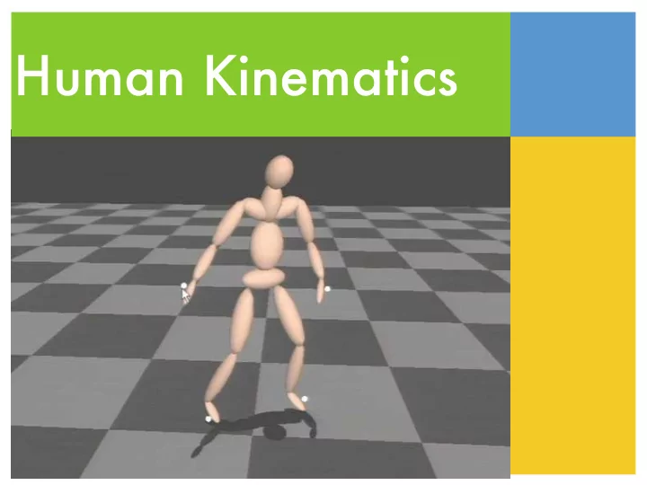
Human Kinematics Kinematic representation Iterative methods - PowerPoint PPT Presentation
Human Kinematics Kinematic representation Iterative methods Optimization methods Motion representation Maximal coordinates Generalized coordinates x, y, z, 0 , 0 , 0 ( x 0 , R 0 ) 1 , 1 ( x 1 , R 1 ) 2 ( x 2 , R 2
Human Kinematics
• Kinematic representation • Iterative methods • Optimization methods
Motion representation Maximal coordinates Generalized coordinates x, y, z, θ 0 , φ 0 , ψ 0 ( x 0 , R 0 ) θ 1 , φ 1 ( x 1 , R 1 ) θ 2 ( x 2 , R 2 ) state variables: 18 state variables: 9 constraints: 9 Assuming there are m links and n DOFs in the articulated body, how many constraints do we need to keep links connected correctly in maximal coordinates?
Maximal coordinates • Direct extension of well understood rigid body dynamics; easy to understand and implement • Operate in Cartesian space; hard to • evaluate joint angles and velocities • enforce joint limits • apply internal joint torques • Inaccuracy in numeric integration can cause body parts to drift apart
Generalized coordinates • Joint space is more intuitive when dealing with complex multi-body structures • Fewer DOFs and fewer constraints • Hard to derive the equation of motion
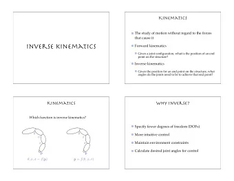
Kinematics • Forward kinematics • given a joint configuration, what is the position of an end point on the structure? • Inverse kinematics • given the position for an end point on the structure, what angles do the joints need be to achieve that end point?
Quiz Which function is inverse kinematics? θ θ φ φ σ σ p p θ , φ , σ = f ( p ) p = f ( θ , φ , σ )
Why inverse? • More intuitive control • Maintain environment constraints • Calculate desired joint angles for control
Motion representation Global position and orientation are determined by 3 translational and 3 rotational DOFs Each joint can have up to 3 DOFs 1 DOF: knee 2 DOF: wrist 3 DOF: arm
Configurations q = x, y, z, θ , φ , σ , θ th , φ th , σ th , θ kn , · · · x, y, z, θ , φ , σ θ thigh , φ thigh , σ thigh θ knee θ ankle , φ ankle
Transformation chain x, y, z, θ , φ , σ d 0 θ thigh , φ thigh , σ thigh d 1 θ knee p d 2 θ ankle , φ ankle h ( q ) h ( q ) = T ( x, y, z ) R ( θ , φ , σ ) T ( d 0 ) R ( θ th , φ th , σ th ) T ( d 1 ) R ( θ kn ) T ( d 2 ) R ( θ an , φ an ) x a point on foot in a point on foot in world coordinates local coordinates
Constraints x, y, z, θ , φ , σ d 0 Position constraint θ thigh , φ thigh , σ thigh d 1 C ( q ) = h ( q ) − p = 0 θ knee p d 2 θ ankle , φ ankle h ( q ) h ( q ) = T ( x, y, z ) R ( θ , φ , σ ) T ( d 0 ) R ( θ th , φ th , σ th ) T ( d 1 ) R ( θ kn ) T ( d 2 ) R ( θ an , φ an ) x a point on foot in a point on foot in world coordinates local coordinates
Solutions • Closed form solutions can only be found for fairly simple mechanisms • Numerical solutions • No solution • Single solution • Multiple solution
Under-specified problem • Multiple solutions • Mostly bad • How do we find the optimal solution? • Heuristics (move the outermost links first) • Closest to the current configuration • Energy minimization • Natural looking motion (whatever it means)
• Kinematic representation • Iterative methods • Optimization methods
Iterative method • Use inverse of Jacobian to iteratively step all the joint angles towards the goal • Girard and Maciejewski, Computational modeling for the computer animation of legged figures, SIGGRAPH 85
Problems • Pseudo inverse returns the least square minimum norm solution • Singularities cause deficient Jacobian • Linearization about current state causes error
• Kinematic representation • Iterative methods • Optimization methods
Optimization method • Find a solution that optimizes some numeric metric and satisfies constraints • Numeric metric • A function of q that measures the quantity to be minimized • Also called “objective function”
Optimization method Solve for joint configuration q min q G ( q ) subject to C ( q ) = 0
Objective functions • Joint velocity • Power consumption • Similarity to the rest pose • Similarity to the natural pose
Unconstrained optimization • Treat each constraint as a separate metric and minimize weighted sum of all metrics • Also called penalty methods • each spring pulls on constraint with force proportional to violation of the constraint
Unconstrained optimization “Softening” constraints by adding them to the objective function Now we have a new optimization problem: � w i C i ( q ) 2 F ( q ) = G ( q ) + min q i
Gradient descent One of the simplest way to solve this optimization is gradient descent method For each iteration, move in the direction of negative gradient T − ∂ F ∂ q = − ∂ G ∂ C i X w i C i ∂ q − 2 ∂ q i q new = q − α∂ F And update the state ∂ q
Optimization loop while F ( q ) > ✏ ∂ q = ∂ G ( q ) ∂ F w i ( ∂ C i compute ∂ q ) T C i X + 2 ∂ q i q = q − α∂ F update ∂ q
Search step size The step size in each search iteration can be determined arbitrarily, through a binary search, or solved by another optimization process Step size: where min α F ( q + α ∆ q ) α q new = q + α ∆ q
Optimize IK problem We can simplify the problem by ignoring G(q), but we still need to know how to compute constraint derivatives. while F ( q ) > ✏ ∂ q = ∂ G ( q ) ∂ F w i ( ∂ C i compute ∂ q ) T C i X + 2 ∂ q i q = q − α∂ F update ∂ q
Constraint derivatives • We need a direction to move joints in such way that the handle moves towards the goal p • The derivative of the constraint, i.e. Jacobian, gives directions h ( q ) where handles move if joints C ( q ) = h ( q ) − p = 0 move ∂ C ( q ) = ∂ h ( q ) ∂ q ∂ q
Quiz • What’s the dimension of the Jacobian for a system with n dofs and m position constraints?
Constraint derivatives C ( q ) = h ( q ) − p = 0 h ( q ) = T ( x, y, z ) R ( θ 0 , φ 0 , σ 0 ) TR ( θ 1 ) TR ( θ 2 , φ 2 ) h k q = [ x, y, z, θ 0 , φ 0 , σ 0 , θ 1 , θ 2 , φ 2 ] x, y, z, ∂ C ( q ) = ∂ h ( q ) θ 0 , φ 0 , σ 0 ∂ q ∂ q ∂ h ( q ) = T ( x, y, z ) R ( θ 0 , φ 0 , σ 0 ) T ∂ R ( θ 1 ) θ 1 TR ( θ 2 , φ 2 ) h k ∂θ 1 ∂θ 1 p θ 2 , φ 2 h ( q ) Need to know how to compute derivatives for each transformation h k : local coordinate of h
Quiz • What is the derivative for the translation matrix? 1 0 0 3 0 1 0 5 0 0 1 − 2 0 0 0 1 • What is the derivative for a rotation matrix about z axis? cos θ sin θ 0 0 − sin θ cos θ 0 0 0 0 1 0 0 0 0 1
Constraint derivatives ∂ h ( q ) What is the most efficient way to compute the ? ∂ q Compute the gradient for the DOF x, y, z, on the outermost link first θ 0 , φ 0 , σ 0 θ 1 h = T 0 ( x, y, z ) R 0 ( θ 0 , φ 0 , σ 0 ) T 1 R 1 ( θ 1 ) T 2 R 2 ( θ 2 , φ 2 ) h k p θ 2 , φ 2 h ( q ) h k : local coordinate of h
Unconstrained optimization • Pros: • simple and fast, no linear system to solve • near-singular configurations is less of a problem • Cons: • can’t maintain constraints exactly • constraints fight against each other and the objective function
Constrained optimization • Treat constraints as “hard constraints” • Use Lagrangian formulation to solve a nonlinear optimization L ( q , λ ) = G ( q ) − λ · C min q , λ L ( q , λ )
Constrained method • Pros • Enforce constraints exactly • Quadratic convergence • Cons • Large system of equations • Near-singular configurations cause instability
Leg example L0 T 0h R(q 0 )R(q 1 )R(q 2 ) hip T h1 L1 T 1k R(q 3 ) knee T k2 L2 T 2a ankle R(q 4 )R(q 5 ) h 0 L3 T a3
Leg example node0 q = {q 0 , q 1 , q 2 , q 3 , q 4 , q 5 } q 0 , q 1 , q 2 hip To evaluate gradients of the obj function at node1 each iteration, we need to evaluate constraint and compute Jacobian. q 3 knee C( q ) = T 0h R 0 R 1 R 2 T h1 T 1k R 3 T k2 T 2a R 4 R 4 T a3 h 0 - p How to compute J( q )? node2 p q 4 , q 5 ankle h 0 node3
Compute Jacobian Consider the derivative of C T 0h R(q 0 )R(q 1 )R(q 2 ) with respect to q 5 T h1 ∂ C = T 0 h R ( q 0 ) R ( q 1 ) R ( q 2 ) T h 1 T 1 k R ( q 3 ) T k 2 T 2 a R ( q 4 ) ∂ R T a 3 h 0 ∂ q 5 ∂ q 5 T 1k R(q 3 ) node->getParentBodyNode()->getTransform() T k2 joint->getTransformFromParentBodyNode() joint T 2a joint->getTransform(0) R(q 4 )R(q 5 ) joint->getTransformDerivative(1) h 0 T a3 joint->getTransformFromChildBodyNode().inverse() node
Recommend
More recommend
Explore More Topics
Stay informed with curated content and fresh updates.
