How to Make a Decision Definitions Based on the Minimum Main - PowerPoint PPT Presentation
Why Minimum Bayes . . . Jeffreys Scale Towards the Precise . . . Formulating the . . . How to Make a Decision Definitions Based on the Minimum Main Result Proof of the Proposition Bayes Factor (MBF): Acknowledgments Bibliography
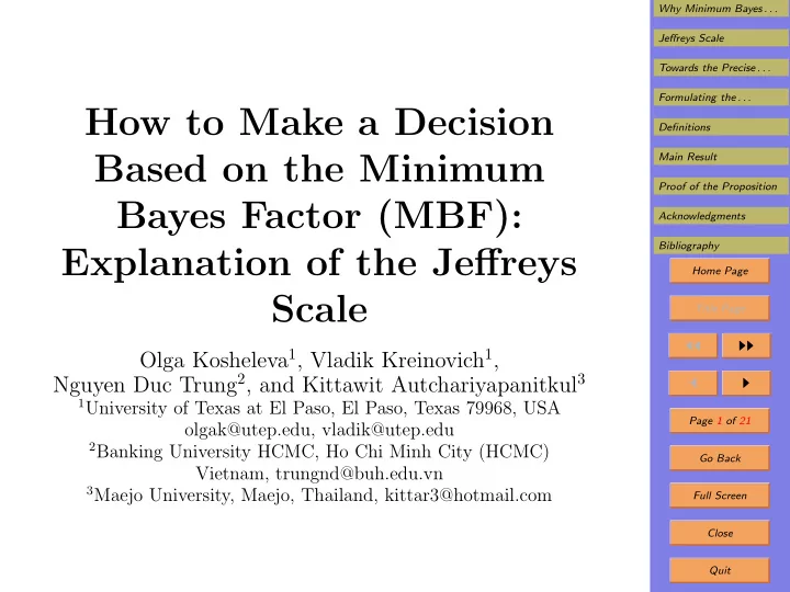
Why Minimum Bayes . . . Jeffreys Scale Towards the Precise . . . Formulating the . . . How to Make a Decision Definitions Based on the Minimum Main Result Proof of the Proposition Bayes Factor (MBF): Acknowledgments Bibliography Explanation of the Jeffreys Home Page Scale Title Page ◭◭ ◮◮ Olga Kosheleva 1 , Vladik Kreinovich 1 , Nguyen Duc Trung 2 , and Kittawit Autchariyapanitkul 3 ◭ ◮ 1 University of Texas at El Paso, El Paso, Texas 79968, USA Page 1 of 21 olgak@utep.edu, vladik@utep.edu 2 Banking University HCMC, Ho Chi Minh City (HCMC) Go Back Vietnam, trungnd@buh.edu.vn 3 Maejo University, Maejo, Thailand, kittar3@hotmail.com Full Screen Close Quit
Why Minimum Bayes . . . Jeffreys Scale 1. Why Minimum Bayes Factor Towards the Precise . . . • In many practical situations: Formulating the . . . Definitions – we have several possible models M i of the corre- Main Result sponding phenomena, and Proof of the Proposition – we would like to decide, based on the data D , which Acknowledgments of these models is more adequate. Bibliography • To select the most appropriate model, statistics text- Home Page books used to recommend techniques based on p-values. Title Page • However, at present: ◭◭ ◮◮ – it is practically a consensus in the statistics com- ◭ ◮ munity Page 2 of 21 – that the use of p-values often results in misleading Go Back conclusions. Full Screen Close Quit
Why Minimum Bayes . . . Jeffreys Scale 2. Why Minimum Bayes Factor (cont-d) Towards the Precise . . . • To make a more adequate selection: Formulating the . . . Definitions – it is important to take prior information into ac- Main Result count, Proof of the Proposition – i.e., to use Bayesian methods. Acknowledgments • It is reasonable to say that the model M 1 is more prob- Bibliography able than the model M 2 if: Home Page – the likelihood P ( D | M 1 ) of getting the data D un- Title Page der the model M 1 is larger than ◭◭ ◮◮ – the likelihood P ( D | M 2 ) of getting the data D un- ◭ ◮ der the model M 2 . Page 3 of 21 = P ( D | M 1 ) def • In other words, the Bayes factor K P ( D | M 2 ) should Go Back exceeds 1. Full Screen Close Quit
Why Minimum Bayes . . . Jeffreys Scale 3. Why Minimum Bayes Factor (cont-d) Towards the Precise . . . • Of course: Formulating the . . . Definitions – if the value is only slightly larger than 1, Main Result – this difference may be caused by the randomness of Proof of the Proposition the corresponding data sample. Acknowledgments • So, in reality, each of the two models can be more ad- Bibliography equate. Home Page • To make a definite conclusion, we need to make sure Title Page that the Bayes factor is sufficiently large. ◭◭ ◮◮ • The larger the factor K , the more confident we are that ◭ ◮ the model M 1 is indeed more adequate. Page 4 of 21 • The numerical value of the Bayes factor K depends on Go Back the prior distribution π : K = K ( π ). Full Screen • In practice, we often do not have enough information to select a single prior distribution. Close Quit
Why Minimum Bayes . . . Jeffreys Scale 4. Why Minimum Bayes Factor (cont-d) Towards the Precise . . . • A more realistic description of the expert’s prior knowl- Formulating the . . . edge is that: Definitions Main Result – we have a family F Proof of the Proposition – of possible prior distributions π . Acknowledgments • In such a situation, we can conclude that the model Bibliography M 1 is more adequate than the model M 2 if: Home Page – the corresponding Bayes factor is sufficiently large Title Page – for all possible prior distributions π ∈ F . ◭◭ ◮◮ def ◭ ◮ • Equivalently, the Minimum Bayes Factor MBF = min π ∈ F K ( π ) should be sufficiently large. Page 5 of 21 Go Back Full Screen Close Quit
Why Minimum Bayes . . . Jeffreys Scale 5. Jeffreys Scale Towards the Precise . . . • In practical applications of Minimum Bayes Factor, the Formulating the . . . following scale is usually used. Definitions Main Result • This scale was originally proposed by Jeffreys in 1989. Proof of the Proposition • When MBF is between 1 and 3, we say that the evi- Acknowledgments dence for the model M 1 is barely worth mentioning. Bibliography Home Page • When the value of MBF is between 3 and 10, we say that the evidence for the model M 1 is substantial. Title Page • When the value of MBF is between 10 and 30, we say ◭◭ ◮◮ that the evidence for the model M 1 is strong. ◭ ◮ • When the value of MBF is between 30 and 100, we say Page 6 of 21 that the evidence for the model M 1 is very strong. Go Back • Finally, when the value of MBF is larger than 100, we Full Screen say that the evidence for the model M 1 is decisive. Close Quit
Why Minimum Bayes . . . Jeffreys Scale 6. Jeffreys Scale (cont-d) Towards the Precise . . . • Jeffreys scale has been effectively used, so it seems to Formulating the . . . be adequate, but why? Definitions Main Result • Why select, e.g., 1 to 3 and not 1 to 2 and 1 to 5? Proof of the Proposition • In this paper, we provide a possible explanation for the Acknowledgments success of Jeffreys scale; this explanation is based on: Bibliography Home Page – a general explanation of the half-order-of-magnitude scales Title Page – provided in our 2006 paper with Jerry Hobbs (USC). ◭◭ ◮◮ ◭ ◮ Page 7 of 21 Go Back Full Screen Close Quit
Why Minimum Bayes . . . Jeffreys Scale 7. Towards the Precise Formulation of the Prob- Towards the Precise . . . lem Formulating the . . . • A scale means, crudely speaking, that: Definitions Main Result – instead of considering all possible values of the MBF, Proof of the Proposition – we consider discretely many values . . . < x 0 < x 1 < Acknowledgments x 2 < . . . corr. to different levels of strength. Bibliography • Every actual value x is then approximated by one of Home Page these values x i ≈ x . Title Page • What is the probability distribution of the resulting ◭◭ ◮◮ def approximation error ∆ x = x i − x ? ◭ ◮ • This error is caused by many different factors. Page 8 of 21 • It is known that under certain reasonable conditions: Go Back – an error caused by many different factors Full Screen – is distributed according to Gaussian (normal) dis- tribution. Close Quit
Why Minimum Bayes . . . Jeffreys Scale 8. Formulating the Problem (cont-d) Towards the Precise . . . • This result – the Central Limit Theorem – is one of the Formulating the . . . reasons why Gaussian distributions are ubiquitous. Definitions Main Result • It is therefore reasonable to assume that ∆ x is normally Proof of the Proposition distributed. Acknowledgments • It is known that a normal distribution is uniquely de- Bibliography termined by its two parameters: Home Page – its average µ and Title Page – its standard deviation σ . ◭◭ ◮◮ • For situations in which the approximating value is x i , ◭ ◮ let us denote: Page 9 of 21 – the mean value of ∆ x by ∆ i , and Go Back – the standard deviation of ∆ x by σ i . Full Screen Close Quit
Why Minimum Bayes . . . Jeffreys Scale 9. Formulating the Problem (cont-d) Towards the Precise . . . • Thus, when the approximate value is x i , the actual Formulating the . . . value x = x i − ∆ x is normally distributed, with: Definitions Main Result – the mean x i − ∆ i (which we will denote by � x i ), and Proof of the Proposition – the standard deviation σ i . Acknowledgments • For a Gaussian distribution, the probability density is Bibliography everywhere positive. Home Page • So, theoretically, we can have values which are as far Title Page away from the mean value µ as possible. ◭◭ ◮◮ • In practice, however, the probabilities of large devia- ◭ ◮ tions from µ are extremely small. Page 10 of 21 • So, the possibility of such deviations can be safely ig- Go Back nored. Full Screen • E.g., the probability of having the value outside the “three sigma” interval [ µ − 3 σ, µ + 3 σ ] is ≈ 0 . 1%. Close Quit
Why Minimum Bayes . . . Jeffreys Scale 10. Formulating the Problem (cont-d) Towards the Precise . . . • Therefore, in most applications, it is assumed that val- Formulating the . . . ues outside this interval are impossible. Definitions Main Result • There are some applications where we cannot make this Proof of the Proposition assumption. Acknowledgments • For example, in designing computer chips, we have mil- Bibliography lions of elements on the chip. Home Page • Then, allowing 0.1% of these elements to malfunction Title Page would mean that: ◭◭ ◮◮ – at any given time, ◭ ◮ – thousands of elements malfunction. Page 11 of 21 • Thus, the chip would malfunction as well. Go Back • For such critical applications, we want the probability Full Screen of deviation to be much smaller, e.g., ≤ 10 − 8 . Close Quit
Recommend
More recommend
Explore More Topics
Stay informed with curated content and fresh updates.
