Homework 2 CSE 573: Artificial Intelligence Autumn 2012 Particle - PDF document

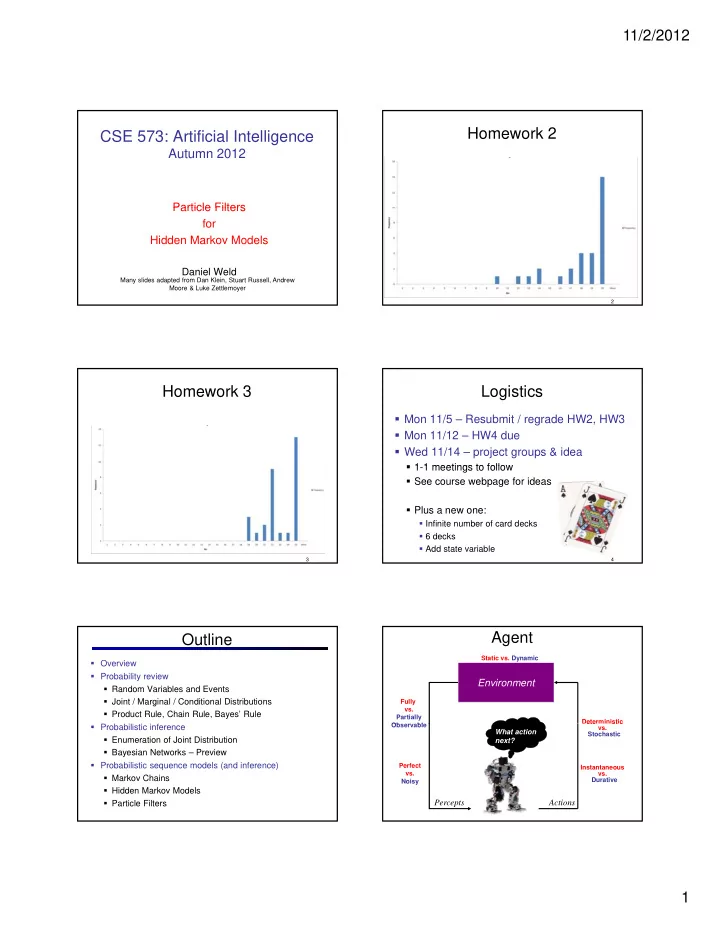
11/2/2012 Homework 2 CSE 573: Artificial Intelligence Autumn 2012 Particle Filters Particle Filters for Hidden Markov Models Daniel Weld Many slides adapted from Dan Klein, Stuart Russell, Andrew Moore & Luke Zettlemoyer 1 2 Homework 3 Logistics  Mon 11/5 – Resubmit / regrade HW2, HW3  Mon 11/12 – HW4 due  Wed 11/14 – project groups & idea  1 1 meetings to follow  1-1 meetings to follow  See course webpage for ideas  Plus a new one:  Infinite number of card decks  6 decks  Add state variable 3 4 Agent Outline Static vs. Dynamic  Overview  Probability review Environment  Random Variables and Events  Joint / Marginal / Conditional Distributions Fully vs.  Product Rule, Chain Rule, Bayes’ Rule Partially Deterministic ete st c  Probabilistic inference Observable Ob bl vs. What action Stochastic  Enumeration of Joint Distribution next?  Bayesian Networks – Preview  Probabilistic sequence models (and inference) Perfect Instantaneous vs. vs.  Markov Chains Durative Noisy  Hidden Markov Models  Particle Filters Percepts Actions 1

11/2/2012 Simple Bayes Net Hidden Markov Model X 1 Hidden Var X 1 X 2 X 3 X 4 X N X 5 Hidden Vars E 1 E 1 E 2 E 3 E 4 E 5 E N Observable Var Observable Vars Defines a joint probability distribution: Defines a joint probability distribution: P(X 1 , E 1 ) = ??? = P(X 1 ) P(E 1 |X 1 ) HMM Computations Real HMM Examples  Given  Part-of-speech (POS) Tagging:  Observations are words (thousands of them)  joint P ( X 1: n , E 1: n )  States are POS tags (eg, noun, verb, adjective, det…)  evidence E 1: n =e 1: n det adj j adj j noun …  Inference problems include:  Filtering, find P ( X t |e 1: n ) for current time n X 1 X 2 X 3 X 4  Smoothing, find P ( X t |e 1: n ) for time t < n  Most probable explanation, find E 1 E 1 E 3 E 4 x* 1: n = argmax x 1: n P ( x 1: n |e 1: n ) The quick brown fox … Real HMM Examples Real HMM Examples  Speech recognition HMMs:  Machine translation HMMs:  Observations are acoustic signals (continuous valued)  States are specific positions in specific words (so, tens of  Observations are words thousands)  States are translation options X 1 X 2 X 3 X 4 X 1 X 2 X 3 X 4 E 1 E 1 E 3 E 4 E 1 E 1 E 3 E 4 2

11/2/2012 Ghostbusters HMM Real HMM Examples 1/9 1/9 1/9  P(X 1 ) = uniform 1/9 1/9 1/9  Robot tracking:  P(X’|X) = usually move clockwise, but sometimes  Observations are range readings (continuous) move in a random direction or stay in place 1/9 1/9 1/9  States are positions on a map (continuous)  P(E|X) = same sensor model as before: P(X 1 ) red means close, green means far away. 1/6 1/6 1/2 X 1 X 2 X 3 X 4 X 1 X 2 X 3 X 4 0 1/6 0 0 0 0 E 1 E 1 E 3 E 4 E 1 E 1 E 3 E 4 P(X’|X=<1,2>) P(red | 3) P(orange | 3) P(yellow | 3) P(green | 3) E 5 P(E|X) 0.05 0.15 0.5 0.3 Filtering aka Monitoring, State Estimation Conditional Independence  Filtering is the task of tracking the distribution B(X) (the HMMs have two important independence properties: belief state) over time  Markov hidden process, future depends on past via the present  Current observation independent of all else given current state  We start with B(X) in an initial setting, usually uniform X 1 X 2 X 3 X 4  As time passes, or we get observations, we update B(X) A ti t b ti d t B(X) E 1 E 1 E 3 E 4  Aside: the Kalman filter  Invented in the 60’s for trajectory estimation in the Apollo program Quiz: does this mean successive observations are independent?  State evolves using a linear model, eg x = x 0 + vt  [No, correlated by the hidden state]  Observe: value of x with Gaussian noise Example: Robot Localization Example: Robot Localization Example from Michael Pfeiffer Prob 0 1 Prob 0 1 t=0 Sensor model: never more than 1 mistake t=1 Motion model: may not execute action with small prob. 3

11/2/2012 Example: Robot Localization Example: Robot Localization 0 1 0 1 Prob Prob t=2 t=3 Example: Robot Localization Example: Robot Localization Prob 0 1 Prob 0 1 t=4 t=5 Inference Recap: Simple Cases Online Belief Updates  Every time step, we start with current P(X | evidence) X 1  We update for time: X 1 X 2 X 1 X 2 E 1 X 2  We update for evidence: E 2 4

11/2/2012 Passage of Time Example: Passage of Time  Assume we have current belief P(X | evidence to date)  As time passes, uncertainty “accumulates” X 1 X 2  Then, after one time step passes:  Or, compactly: T = 1 T = 2 T = 5  Basic idea: beliefs get “pushed” through the transitions  With the “B” notation, we have to be careful about what time step t the belief is about, and what evidence it includes Transition model: ghosts usually go clockwise Observation Example: Observation  Assume we have current belief P(X | previous evidence):  As we get observations, beliefs get reweighted, uncertainty “decreases” X 1  Then: E 1  Or: Before observation After observation  Basic idea: beliefs reweighted by likelihood of evidence  Unlike passage of time, we have to renormalize The Forward Algorithm Example: Run the Filter  We want to know:  We can derive the following updates  An HMM is defined by:  Initial distribution:  Transitions:  To get , compute each entry and normalize  Emissions: 5

11/2/2012 Example HMM Example Pac-man Summary: Filtering Recap: Reasoning Over Time 0.3  Filtering is the inference process of finding a distribution  Stationary Markov models 0.7 over X T given e 1 through e T : P( X T | e 1:t ) rain sun X 1 X 2 X 3 X 4 0.7 0.3  We first compute P( X 1 | e 1 ):  For each t from 2 to T, we have P( X t-1 | e 1:t-1 )  Elapse time: compute P( X t | e 1:t-1 )  Hidden Markov models X E P rain umbrella 0.9 X 1 X 2 X 3 X 4 X 5  Observe: compute P(X t | e 1:t-1 , e t ) = P( X t | e 1:t ) rain no umbrella 0.1 sun umbrella 0.2 E 1 E 2 E 3 E 4 E 5 sun no umbrella 0.8 Add a slide Particle Filtering  Sometimes |X| is too big to use exact  Next slide (intro to particle filtering) is 0.0 0.1 0.0 inference  |X| may be too big to even store B(X) confusing because the state spaec is so 0.0 0.0 0.2  E.g. when X is continuous small – show a huge grid, where it’s clear  |X| 2 may be too big to do updates 0.0 0.2 0.5 what advantage one gets. what advantage one gets  Solution: approximate inference  Maybe also introduce parametric  Track samples of X, not all values  Samples are called particles representations (kalman filter) here  Time per step is linear in the number of samples  But: number needed may be large  In memory: list of particles, not states  This is how robot localization works in practice 37 6

11/2/2012 Representation: Particles Particle Filtering: Elapse Time  Each particle is moved by sampling  Our representation of P(X) is now a list of N particles (samples) its next position from the transition  model Generally, N << |X|  Storing map from X to counts would defeat the point   This is like prior sampling – samples’ P(x) approximated by number of Particles: particles with value x frequencies reflect the transition probs (3,3)  Here, most samples move clockwise, but  (2,3) So, many x will have P(x) = 0! (3,3) some move in another direction or stay in  More particles, more accuracy (3,2) place (3,3) (3,2)  For now, all particles have a (2,1)  This captures the passage of time (3,3) weight of 1 (3,3)  If we have enough samples, close to the (2,1) exact values before and after (consistent) Particle Filtering: Observe Particle Filtering: Observe  Slightly trickier:  Instead of sampling the observation…  Use P(e|x) to sample observation, and  Fix It!  Discard particles which are inconsistent?  A kind of likelihood weighting  (Called Rejection Sampling)  Downweight samples based on evidence  Problems?  Note that probabilities don’t sum to one: (most have been down-weighted) Instead, they sum to an approximation of P(e))  What to do?!? Particle Filtering: Resample Recap: Particle Filtering At each time step t, we have a set of N particles (aka samples) Old Particles:  Rather than tracking (3,3) w=0.1  Initialization: Sample from prior weighted samples, (2,1) w=0.9 (2,1) w=0.9 we resample – why?  Three step procedure for moving to time t+1: (3,1) w=0.4 (3,2) w=0.3 1. Sample transitions: for each each particle x , sample next (2,2) w=0.4  N times, we choose state (1,1) w=0.4 from our weighted (3,1) w=0.4 sample distribution sample distribution (2,1) w=0.9 (2 1) 0 9 (i.e. draw with (3,2) w=0.3 replacement) 2. Reweight: for each particle, compute its weight given the New Particles: actual observation e (2,1) w=1  This is equivalent to (2,1) w=1 renormalizing the (2,1) w=1 (3,2) w=1 distribution 3. Resample: normalize the weights, and sample N new (2,2) w=1 (2,1) w=1 particles from the resulting distribution over states  (1,1) w=1 Now the update is (3,1) w=1 complete for this time (2,1) w=1 step, continue with (1,1) w=1 the next one 7