Hoeffdings Bound Theorem Let X 1 , . . . , X n be independent random - PowerPoint PPT Presentation

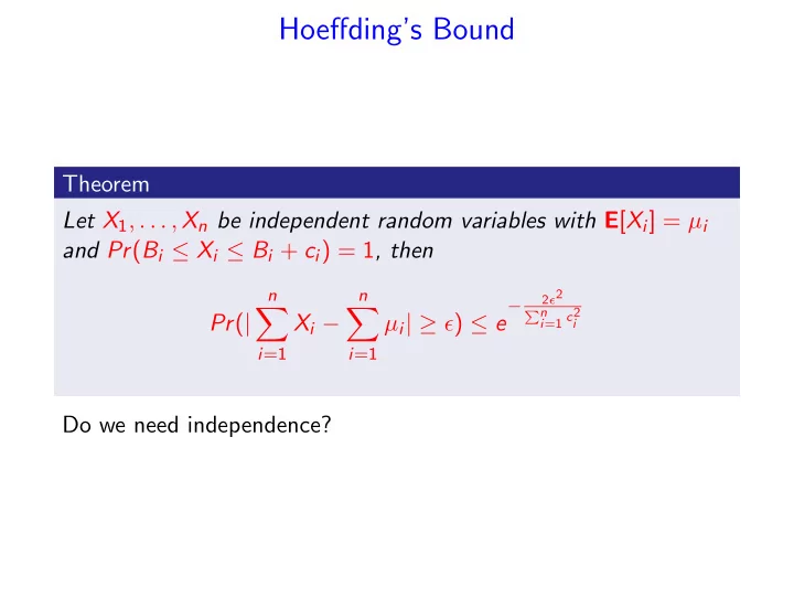
Hoeffding’s Bound Theorem Let X 1 , . . . , X n be independent random variables with E [ X i ] = µ i and Pr ( B i ≤ X i ≤ B i + c i ) = 1 , then n n 2 ǫ 2 − � � i =1 c 2 � n Pr ( | X i − µ i | ≥ ǫ ) ≤ e i i =1 i =1 Do we need independence?

Martingales Definition A sequence of random variables Z 0 , Z 1 , . . . is a martingale with respect to the sequence X 0 , X 1 , . . . if for all n ≥ 0 the following hold: 1 Z n is a function of X 0 , X 1 , . . . , X n ; 2 E [ | Z n | ] < ∞ ; 3 E [ Z n +1 | X 0 , X 1 , . . . , X n ] = Z n ; Definition A sequence of random variables Z 0 , Z 1 , . . . is a martingale when it is a martingale with respect to itself, that is 1 E [ | Z n | ] < ∞ ; 2 E [ Z n +1 | Z 0 , Z 1 , . . . , Z n ] = Z n ;

Conditional Expectation Definition � E [ Y | Z = z ] = y Pr( Y = y | Z = z ) , y where the summation is over all y in the range of Y . Lemma For any random variables X and Y , � E [ X ] = E Y [ E X [ X | Y ]] = Pr( Y = y ) E [ X | Y = y ] , y where the sum is over all values in the range of Y .

Lemma For any random variables X and Y , � E [ X ] = E Y [ E X [ X | Y ]] = Pr( Y = y ) E [ X | Y = y ] , y where the sum is over all values in the range of Y . Proof. � Pr( Y = y ) E [ X | Y = y ] y � � = Pr( Y = y ) x Pr( X = x | Y = y ) y x � � = x Pr( X = x | Y = y ) Pr( Y = y ) x y � � � = x Pr( X = x ∩ Y = y ) = x Pr( X = x ) = E [ X ] . x y x

Example Consider a two phase game: • Phase I: roll one die. Let X be the outcome. • Phase II: Flip X fair coins, let Y be the number of HEADs. • You receive a dollar for each HEAD. Y is distributed B ( X , 1 2 ), E [ Y | X = a ] = a 2 6 � E [ Y ] = E [ Y | X = i ] Pr( X = i ) i =1 6 2 Pr( X = i ) = 7 i � = 4 i =1

Conditional Expectation as a Random variable Definition The expression E [ Y | Z ] is a random variable f ( Z ) that takes on the value E [ Y | Z = z ] when Z = z . Consider the outcome of rolling two dice X 1 , X 2 , X = X 1 + X 2 . X 1 +6 x · 1 6 = X 1 + 7 � � E [ X | X 1 ] = x Pr( X = x | X 1 ) = 2 . x x = X 1 +1 Consider the two phase game E [ Y | X ] = X 2

If E [ Y | Z ] is a random variable, it has an expectation. Theorem E [ Y ] = E [ E [ Y | Z ]] . E [ X | X 1 ] = X 1 + 7 2 . Thus � X 1 + 7 � = 7 2 + 7 E [ E [ X | X 1 ]] = E 2 = 7 . 2

Martingales Definition A sequence of random variables Z 0 , Z 1 , . . . is a martingale with respect to the sequence X 0 , X 1 , . . . if for all n ≥ 0 the following hold: 1 Z n is a function of X 0 , X 1 , . . . , X n ; 2 E [ | Z n | ] < ∞ ; 3 E [ Z n +1 | X 0 , X 1 , . . . , X n ] = Z n ; Definition A sequence of random variables Z 0 , Z 1 , . . . is a martingale when it is a martingale with respect to itself, that is 1 E [ | Z n | ] < ∞ ; 2 E [ Z n +1 | Z 0 , Z 1 , . . . , Z n ] = Z n ;

Martingale Example A series of fair games ( E [gain] = 0), not necessarily independent.. Game 1: bet $1. Game i > 1: bet 2 i if won in round i − 1; bet i otherwise. X i = amount won in i th game. ( X i < 0 if i th game lost). Z i = total winnings at end of i th game.

Example X i = amount won in i th game. ( X i < 0 if i th game lost). Z i = total winnings at end of i th game. Z 1 , Z 2 , . . . is martingale with respect to X 1 , X 2 , . . . E [ X i ] = 0 . E [ Z i ] = � E [ X i ] = 0 < ∞ . E [ Z i +1 | X 1 , X 2 , . . . , X i ] = Z i + E [ X i +1 ] = Z i .

Gambling Strategies I play series of fair games (win with probability 1 / 2). Game 1: bet $1. Game i > 1: bet 2 i if I won in round i − 1; bet i otherwise. X i = amount won in i th game. ( X i < 0 if i th game lost). Z i = total winnings at end of i th game. Assume that (before starting to play) I decide to quit after k games: what are my expected winnings?

Lemma Let Z 0 , Z 1 , Z 2 , . . . be a martingale with respect to X 0 , X 1 , . . . . For any fixed n, E X [1: n ] [ Z n ] = E [ Z 0 ] . (X [1 : i ] = X 1 , . . . , X i ) Proof. Since Z i is a martingale Z i − 1 = E X i [ Z i | X 0 , X 1 , . . . , X i − 1 ] . Then E X [1: i − 1] [ Z i − 1 ] = E X [1: i − 1] [ E X i [ Z i | X 0 , X 1 , . . . , X i − 1 ]] But E X [1: i − 1] [ E X i [ Z i | X 0 , X 1 , . . . , X i − 1 ]] = E X [1: i ] [ Z i ] . Thus, E X [1: n ] [ Z n ] = E X [ n − 1] [ Z n − 1 ] = . . . , = E [ Z 0 ] .

Gambling Strategies I play series of fair games (win with probability 1 / 2). Game 1: bet $1. Game i > 1: bet 2 i if I won in round i − 1; bet i otherwise. X i = amount won in i th game. ( X i < 0 if i th game lost). Z i = total winnings at end of i th game. Assume that (before starting to gamble) we decide to quit after k games: what are my expected winnings? E [ Z k ] = E [ Z 1 ] = 0.

A Different Strategy Same gambling game. What happens if I: • play a random number of games? • decide to stop only when I have won $1000?

Stopping Time Definition A non-negative, integer random variable T is a stopping time for the sequence Z 0 , Z 1 , . . . if the event “ T = n ” depends only on the value of random variables Z 0 , Z 1 , . . . , Z n . Intuition: corresponds to a strategy for determining when to stop a sequence based only on values seen so far. In the gambling game: • first time I win 10 games in a row : is a stopping time; • the last time when I win : is not a stopping time.

Consider again the gambling game: let T be a stopping time. Z i = total winnings at end of i th game. What are my winnings at the stopping time, i.e. E [ Z T ]? Fair game: E [ Z T ] = E [ Z 0 ] = 0? “ T =first time my total winnings are at least $1000” is a stopping time, and E [ Z T ] > 1000...

Martingale Stopping Theorem Theorem If Z 0 , Z 1 , . . . is a martingale with respect to X 1 , X 2 , . . . and if T is a stopping time for X 1 , X 2 , . . . then E [ Z T ] = E [ Z 0 ] whenever one of the following holds: • there is a constant c such that, for all i, | Z i | ≤ c; • T is bounded; • E [ T ] < ∞ , and there is a constant c such that � � � E | Z i +1 − Z i | � X 1 , . . . , X i < c.

Proof of Martingale Stopping Theorem (Sketch) We need to show that E [ | Z T | ] < ∞ . So we can use E [ Z T ] = E [ Z 0 ] + � i ≤ T E [ E [( Z i − Z i − 1 ) | X 1 , . . . , X i − 1 ]] • there is a constant c such that, for all i , | Z i | ≤ c - the sum is bounded. • T is bounded - the sum has finite number of elements. • E [ T ] < ∞ , and there is a constant c such that � � � E | Z i +1 − Z i | � X 1 , . . . , X i < c ∞ � � � � E [ | Z T | ] ≤ E [ | Z 0 | ] + E [ E | Z i +1 − Z i | � X 1 , . . . , X i 1 i ≤ T ] i =1 ∞ � ≤ E [ | Z 0 | ] + c Pr ( T ≥ i ) i =1 ≤ E [ | Z 0 | ] + cE [ T ] < ∞

Martingale Stopping Theorem Applications We play a sequence of fair game with the following stopping rules: 1 T is chosen from distribution with finite expectation: E [ Z T ] = E [ Z 0 ]. 2 T is the first time we made $1000: E [ T ] is unbounded. 3 We double until the first win. E [ T ] = 2 but � � � E | Z i +1 − Z i | � X 1 , . . . , X i is unbounded.

Example: The Gambler’s Ruin • Consider a sequence of independent, fair 2-player gambling games. • In each round, each player wins or loses $1 with probability 1 2 . • X i = amount won by player 1 on i th round. • If player 1 has lost in round i : X i < 0. • Z i = total amount won by player 1 after i th rounds. • Z 0 = 0. • Game ends when one player runs out of money • Player 1 must stop when she loses net ℓ 1 dollars ( Z t = − ℓ 1 ) • Player 2 terminates when she loses net ℓ 2 dollars ( Z t = ℓ 2 ). • q = probability game ends with player 1 winning ℓ 2 dollars.

Example: The Gambler’s Ruin • T = first time player 1 wins ℓ 2 dollars or loses ℓ 1 dollars. • T is a stopping time for X 1 , X 2 , . . . . • Z 0 , Z 1 , . . . is a martingale. • Z i ’s are bounded. • Martingale Stopping Theorem: E [ Z T ] = E [ Z 0 ] = 0. E [ Z T ] = q ℓ 2 − (1 − q ) ℓ 1 = 0 ℓ 1 q = ℓ 1 + ℓ 2

Example: A Ballot Theorem • Candidate A and candidate B run for an election. • Candidate A gets a votes. • Candidate B gets b votes. • a > b . • Votes are counted in random order : • chosen from all permutations on all n = a + b votes. • What is the probability that A is always ahead in the count?

Example: A Ballot Theorem • S i = number of votes A is leading by after i votes counted • If A is trailing: S i < 0). • S n = a − b . • For 0 ≤ k ≤ n − 1: X k = S n − k n − k . • Consider X 0 , X 1 , . . . , X n . • This sequence goes backward in time! E [ X k | X 0 , X 1 , . . . , X k − 1 ] = ?

Example: A Ballot Theorem E [ X k | X 0 , X 1 , . . . , X k − 1 ] = ? • Conditioning on X 0 , X 1 , . . . , X k − 1 : equivalent to conditioning on S n , S n − 1 , . . . , S n − k +1 , • a i = number of votes for A after first i votes are counted. • ( n − k + 1)th vote: random vote among these first n − k + 1 votes. � S n − k +1 + 1 if ( n − k + 1)th vote is for B S n − k = S n − k +1 − 1 if ( n − k + 1)th vote is for A � with prob. n − k +1 − a n − k +1 S n − k +1 + 1 n − k +1 S n − k = a n − k +1 S n − k +1 − 1 with prob. n − k +1