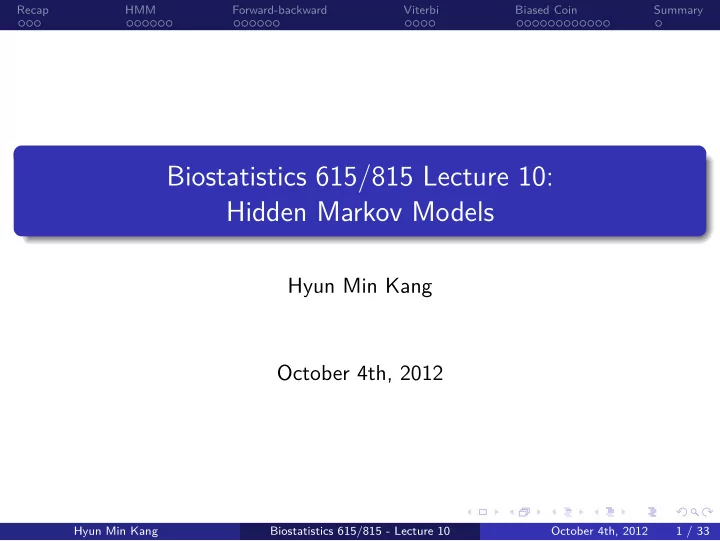
Hidden Markov Models Biostatistics 615/815 Lecture 10: . . - PowerPoint PPT Presentation

. Biased Coin October 4th, 2012 Biostatistics 615/815 - Lecture 10 Hyun Min Kang October 4th, 2012 Hyun Min Kang Hidden Markov Models Biostatistics 615/815 Lecture 10: . . Summary . 1 / 33 . Viterbi Forward-backward HMM Recap . . . . . . . . . . . . . . . . . . . . . . . . . . . . . . . . . . .

. Viterbi October 4th, 2012 Biostatistics 615/815 - Lecture 10 Hyun Min Kang computation. min . Manhattan Tourist Problem Summary . Biased Coin 2 / 33 . . . . Forward-backward HMM . . . Recap . . . . . . . . . . . . . . . . . . . . . . . . . . . . • Let C ( r , c ) be the optimal cost from (0 , 0) to ( r , c ) • Let h ( r , c ) be the weight from ( r , c ) to ( r , c + 1) • Let v ( r , c ) be the weight from ( r , c ) to ( r + 1 , c ) • We can recursively define the optimal cost as  { C ( r − 1 , c ) + v ( r − 1 , c ) r > 0 , c > 0   C ( r , c − 1) + h ( r , c − 1)    C ( r , c ) = C ( r , c − 1) + h ( r , c − 1) r = 0 , c > 0 C ( r − 1 , c ) + v ( r − 1 , c ) r > 0 , c = 0     0 r = 0 , c = 0  • Once C ( r , c ) is evaluated, it must be stored to avoid redundant

. . October 4th, 2012 Biostatistics 615/815 - Lecture 10 Hyun Min Kang Edit Distance Problem Summary . Biased Coin Viterbi Forward-backward HMM Recap . . . . . . . 3 / 33 . . . . . . . . . . . . . . . . . . . . . . . . . . . .

. Biased Coin October 4th, 2012 Biostatistics 615/815 - Lecture 10 Hyun Min Kang otherwise min j i . Dynamic Programming for Edit Distance Problem Summary . 4 / 33 HMM Forward-backward . . . . . . . Recap Viterbi . . . . . . . . . . . . . . . . . . . . . . . . . . . . • Input strings are x [1 , · · · , m ] and y [1 , · · · , n ] . • Let x i = x [1 , · · · , i ] and y j = y [1 , · · · , j ] be substrings of x and y . • Edit distance d ( x , y ) can be recursively defined as follows  j = 0   i = 0      d ( x i , y j ) = d ( x i − 1 , y j ) + 1   d ( x i , y j − 1 ) + 1      d ( x i − 1 , y i − 1 ) + I ( x [ i ] ̸ = y [ j ])   • Similar to the Manhattan tourist problem, but with 3-way choice. • Time complexity is Θ( mn ) .

. Viterbi October 4th, 2012 Biostatistics 615/815 - Lecture 10 Hyun Min Kang states can be obtained. Markov process Hidden Markov Models (HMMs) Summary . Biased Coin . 5 / 33 Forward-backward HMM Recap . . . . . . . . . . . . . . . . . . . . . . . . . . . . . . . . . . . • A Markov model where actual state is unobserved • Transition between states are probabilistically modeled just like the • Typically there are observable outputs associated with hidden states • The probability distribution of observable outputs given an hidden

. Viterbi October 4th, 2012 Biostatistics 615/815 - Lecture 10 Hyun Min Kang . An example of HMM Summary . Biased Coin 6 / 33 Forward-backward HMM Recap . . . . . . . . . . . . . . . . . . . . . . . . . . . . . . . . . . . 345$ 348$ 346$ !"#!$ %&'$ 347$ 3466$ 3493$ ()**+$ 3493$ 3483$ ,-.)/+$ 3435$ 34:3$ 012*+$ • Direct Observation : (SUNNY, CLOUDY, RAINY) • Hidden States : (HIGH, LOW)

S i , S j q t b q t o t b S i O j O j q t . S i Initial States i Pr q Transition A ij Pr q t Emission B ij A O Pr o t S i B Hyun Min Kang Biostatistics 615/815 - Lecture 10 October 4th, 2012 (SUNNY, CLOUDY, RAINY) O . O . . . . . . . Recap HMM Forward-backward Viterbi Biased Coin . Summary Mathematical representation of the HMM example Outcomes O 7 / 33 . . . . . . . . . . . . . . . . . . . . . . . . . . . . States S = { S 1 , S 2 } = (HIGH, LOW)

S i , S j q t b q t o t b S i O j O j q t A Pr q Transition A ij Pr q t S i . Emission B ij Initial States Pr o t S i B Hyun Min Kang Biostatistics 615/815 - Lecture 10 October 4th, 2012 i 7 / 33 . . Mathematical representation of the HMM example Summary . Biased Coin . Viterbi . Forward-backward . HMM Recap . . . . . . . . . . . . . . . . . . . . . . . . . . . . . . . States S = { S 1 , S 2 } = (HIGH, LOW) Outcomes O = { O 1 , O 2 , O 3 } = (SUNNY, CLOUDY, RAINY)

S j q t b q t o t b S i O j O j q t . Pr q t S i A Emission B ij Pr o t . S i B Hyun Min Kang Biostatistics 615/815 - Lecture 10 October 4th, 2012 Transition A ij 7 / 33 Mathematical representation of the HMM example . . . . . . Biased Coin . Viterbi . Forward-backward Summary HMM Recap . . . . . . . . . . . . . . . . . . . . . . . . . . . . States S = { S 1 , S 2 } = (HIGH, LOW) Outcomes O = { O 1 , O 2 , O 3 } = (SUNNY, CLOUDY, RAINY) Initial States π i = Pr ( q 1 = S i ) , π = { 0 . 7 , 0 . 3 }

. Viterbi October 4th, 2012 Biostatistics 615/815 - Lecture 10 Hyun Min Kang . Mathematical representation of the HMM example Summary . Biased Coin 7 / 33 Forward-backward HMM Recap . . . . . . . . . . . . . . . . . . . . . . . . . . . . . . . . . . . States S = { S 1 , S 2 } = (HIGH, LOW) Outcomes O = { O 1 , O 2 , O 3 } = (SUNNY, CLOUDY, RAINY) Initial States π i = Pr ( q 1 = S i ) , π = { 0 . 7 , 0 . 3 } Transition A ij = Pr ( q t +1 = S j | q t = S i ) ( 0 . 8 ) 0 . 2 A = 0 . 4 0 . 6 Emission B ij = b q t ( o t ) = b S i ( O j ) = Pr ( o t = O j | q t = S i ) ( 0 . 88 ) 0 . 10 0 . 02 B = 0 . 10 0 . 60 0 . 30

. Biased Coin October 4th, 2012 Biostatistics 615/815 - Lecture 10 Hyun Min Kang The chance of rain in day 4 is 23.3% . . . What is the chance of rain in the day 4? . Unconditional marginal probabilities Summary . 8 / 33 Viterbi . Forward-backward HMM Recap . . . . . . . . . . . . . . . . . . . . . . . . . . . . . . . . . . ( 0 . 669 ( Pr ( q 4 = S 1 ) ) ) = ( A T ) 3 π = f ( q 4 ) = Pr ( q 4 = S 2 ) 0 . 331     Pr ( o 4 = O 1 ) 0 . 621  = B T f ( q 4 ) = g ( o 4 ) = Pr ( o 4 = O 2 ) 0 . 266    Pr ( o 4 = O 3 ) 0 . 233

. Biased Coin October 4th, 2012 Biostatistics 615/815 - Lecture 10 Hyun Min Kang t q t t . q Marginal likelihood of data in HMM Summary . t 9 / 33 HMM Forward-backward . . . . . . . Recap Viterbi . . . . . . . . . . . . . . . . . . . . . . . . . . . . • Let λ = ( A , B , π ) • For a sequence of observation o = { o 1 , · · · , o t } , ∑ Pr ( o | λ ) = Pr ( o | q , λ ) Pr ( q | λ ) ∏ ∏ Pr ( o | q , λ ) = Pr ( o i | q i , λ ) = b q i ( o i ) i =1 i =1 ∏ Pr ( q | λ ) = π q 1 a q i − 1 q i i =2 ∑ ∏ Pr ( o | λ ) = π q 1 b q 1 ( o 1 ) a q i − 1 q i b q i ( o i ) i =2

. Viterbi October 4th, 2012 Biostatistics 615/815 - Lecture 10 Hyun Min Kang of observations t q Naive computation of the likelihood . . Biased Coin Summary 10 / 33 . Forward-backward HMM . . Recap . . . . . . . . . . . . . . . . . . . . . . . . . . . . . . . . ∑ ∏ Pr ( o | λ ) = π q 1 b q 1 ( o 1 ) a q i − 1 q i b q i ( o i ) i =2 • Number of possible q = 2 t are exponentially growing with the number • Computational would be infeasible for large number of observations • Algorithmic solution required for efficient computation.

. . October 4th, 2012 Biostatistics 615/815 - Lecture 10 Hyun Min Kang each day? from day 1 through day 5, what is the distribution of hidden states for More Markov Chain Question Summary . Biased Coin Viterbi Forward-backward HMM Recap . . . . . . . 11 / 33 . . . . . . . . . . . . . . . . . . . . . . . . . . . . • If the observation was (SUNNY,SUNNY,CLOUDY,RAINY,RAINY) • Need to know Pr ( q t | o , λ )

. Viterbi October 4th, 2012 Biostatistics 615/815 - Lecture 10 Hyun Min Kang . t t Forward and backward probabilities Summary . Biased Coin 12 / 33 . . Forward-backward HMM . Recap . . . . . . . . . . . . . . . . . . . . . . . . . . . . . . . . q + = ( q 1 , · · · , q t − 1 ) , t = ( q t +1 , · · · , q T ) q − o + = ( o 1 , · · · , o t − 1 ) , t = ( o t +1 , · · · , o T ) o − Pr ( q t = i , o | λ ) Pr ( q t = i , o | λ ) Pr ( q t = i | o , λ ) = = Pr ( o | λ ) ∑ n j =1 Pr ( q t = j , o | λ ) t , o t , o + Pr ( q t , o | λ ) = Pr ( q t , o − t | λ ) Pr ( o + = t | q t , λ ) Pr ( o − t | q t , λ ) Pr ( o t | q t , λ ) Pr ( q t | λ ) Pr ( o + = t | q t , λ ) Pr ( o − t , o t , q t | λ ) = β t ( q t ) α t ( q t ) If α t ( q t ) and β t ( q t ) is known, Pr ( q t | o , λ ) can be computed in a linear time.

. Biased Coin October 4th, 2012 Biostatistics 615/815 - Lecture 10 Hyun Min Kang n n n . DP algorithm for calculating forward probability Summary . 13 / 33 Viterbi . . . . Recap . . . Forward-backward HMM . . . . . . . . . . . . . . . . . . . . . . . . . . . . • Key idea is to use ( q t , o t ) ⊥ o − t | q t − 1 . • Each of q t − 1 , q t , and q t +1 is a Markov blanket. α t ( i ) = Pr ( o 1 , · · · , o t , q t = i | λ ) ∑ = Pr ( o − t , o t , q t − 1 = j , q t = i | λ ) j =1 ∑ = Pr ( o − t , q t − 1 = j | λ ) Pr ( q t = i | q t − 1 = j , λ ) Pr ( o t | q t = i , λ ) j =1 ∑ = α t − 1 ( j ) a ji b i ( o t ) j =1 α 1 ( i ) = π i b i ( o 1 )