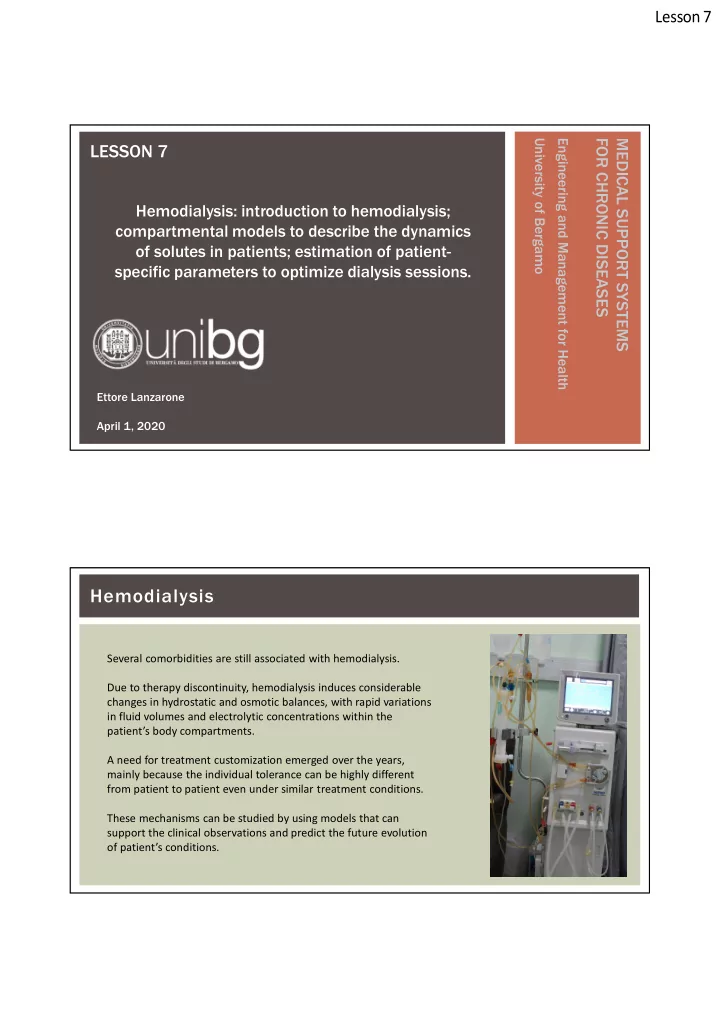
Hemodialysis Several comorbidities are still associated with - PDF document

Lesson 7 University of Bergamo Engineering and Management for Health FOR CHRONIC DISEASES MEDICAL SUPPORT SYSTEMS LESSON 7 Hemodialysis: introduction to hemodialysis; compartmental models to describe the dynamics of solutes in patients; estimation of patient- specific parameters to optimize dialysis sessions. Ettore Lanzarone April 1, 2020 Hemodialysis Several comorbidities are still associated with hemodialysis. Due to therapy discontinuity, hemodialysis induces considerable changes in hydrostatic and osmotic balances, with rapid variations in fluid volumes and electrolytic concentrations within the patient’s body compartments. A need for treatment customization emerged over the years, mainly because the individual tolerance can be highly different from patient to patient even under similar treatment conditions. These mechanisms can be studied by using models that can support the clinical observations and predict the future evolution of patient’s conditions.

Lesson 7 Hemodialysis More specifically, a proper mathematical model of fluid exchange and solute dynamics would provide the clinicians an instrument to simulate and predict the single-patient response to the treatment in terms of solutes and catabolite kinetics, so as to identify the most suitable therapy, thereby reducing intradialysis complications and associated longterm dysfunctions. Hemodialysis We consider the parametric multicompartmental model of Casagrande et al. (2016) that accounts for several solutes and allows to include the patient-specific characteristics through a proper setting of the parameters. In our course: • Description of the model • Approaches to obtain patient-specific parameters Casagrande et al. Patient-specific modeling of multicompartmental fluid and mass exchange during dialysis. The International Journal of Artificial Organs 2016; 39(5): 220-227

Lesson 7 Hemodialysis MODEL • Multi-compartmental parametric kinetic model based on mass and fluid balance equations both in the patient and across the dialyzer membrane. • Dynamics determined by balance equations for hydraulic and osmotic pressures in the patient. • Body compartments are represented as 2 pools for the mass exchange analysis of the solutes (intracellular and extracellular) and as 3 pools (plasmatic, interstitial and intracellular) for fluids transfer. Hemodialysis MODEL Simultaneous evaluation of the temporal trend in patient’s blood of: • plasmatic electrolytes, e.g., Sodium (Na+), Potassium (K+), Chloride (Cl-), Calcium (Ca2+), Bicarbonate (HCO3-) and Magnesium (Mg2+); • breakdown products, e.g., creatinine and urea; • protein concentrations.

Lesson 7 Hemodialysis • Overview of the main components • Resulting system • Estimation of patient- specific parameters Hemodialysis Dialyzer-side equations

Lesson 7 Hemodialysis Dialyzer-side equations Hemodialysis Dialyzer-side equations

Lesson 7 Hemodialysis Patient-side equations Hemodialysis Patient-side equations

Lesson 7 Hemodialysis Patient-side equations Hemodialysis Patient-side equations

Lesson 7 Hemodialysis Patient-side equations Hemodialysis Summing up, mass, the considered mathematical model includes mass, fluid and pressure balance equations that account for mass and fluid exchanges in the body compartments. 1) • ( s ) : mass of solute s in the intracellular M ic compartment • ( s ) : mass of solute s in the extracellular M ex compartment

Lesson 7 Hemodialysis Summing up, mass, the considered mathematical model includes mass, fluid and pressure balance equations that account for mass and fluid exchanges in the body compartments. 2) • V ic : fluid volume in the intracellular compartment • V is : fluid volume in the interstitial compartment • V pl : fluid volume in the plasmatic compartment Hemodialysis Summing up, mass, the considered mathematical model includes mass, fluid and pressure balance equations that account for mass and fluid exchanges in the body compartments. 3) • P ac : pressure at the arterial capillary side • P is : pressure in the interstitial compartment

Lesson 7 Hemodialysis The other variables that vary over time are expressed in function of the above mentioned state variables, with no additional differential equations (Bianchi et al. 2017). The model includes two types of parameters (Bianchi et al. 2017): - Fixed parameters - Patient-specific parameters Hemodialysis All the mass, fluid and pressure balance equations compose a system of Ordinary Differential Equations (ODE), which is numerically solved by the 4th-order Runge-Kutta numerical method. Practical lesson The goals are: 1. To estimate the coefficients under a frequentist approach (e.g., MLE) 2. To estimate the coefficients under the Bayesian approach I provide you: • Matlab code with the Runge-Kutta discretization • Some datasets • RSTAN model for Bayesian estimation [ later in lesson 9 for goal 2 ]

Lesson 7 Hemodialysis Matlab code with the Runge-Kutta discretization FOCUS ON THIS PART Hemodialysis • Tasks for the frequentist estimation: 1. To run the model to generate a simulated dataset with a given set of patient-specific parameters (you can keep those written in the file). 2. To forget these parameters and to develop a method to re-estimate them; suggestion provided in the next slides.

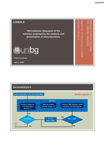
Lesson 7 Hemodialysis 3. To apply the method you proposed to the real patient dataset you can find in the text file “patient.csv” Time step of the acquisitions is 1 minute. Pay attention to the fact that there are missing osbservations (those with -1). Some variables are observed only at the beginning and the end Hemodialysis Suggestion: ITERATIVE APPROACH

Lesson 7 Hemodialysis A suitable approach is to minimize one of the validation metrics where the considered points are the observations available in the dataset. As the model is complex and nonlinear, an iterative approach is suggested. Hemodialysis Iteration block Choose a set θ of Simulate outputs Compute MSE between model parameters with the chosen set outcomes and observations

Lesson 7 Hemodialysis Initial reasonable θ 0 with associated MSE 0 Feedback Iteration i Choose a newer set Simulate outputs Compute MSE i between model θ i of parameters with the chosen set outcomes and observations based on θ * YES θ * = θ i MSE i < MSE * MSE * = MSE i ? NO Hemodialysis Initial reasonable θ 0 with associated MSE 0 Iterative approach Iteration i Simulate outputs Compute MSE i between model Choose a newer set θ i of parameters with the chosen set outcomes and observations based on θ * NO YES Terminate θ * = θ i MSE i < MSE * ? MSE * = MSE i ? θ * NO YES

Lesson 7 Hemodialysis Try to implement and test