Hectors & Mui dolphin TMP risk assessment Risk assessment - PowerPoint PPT Presentation
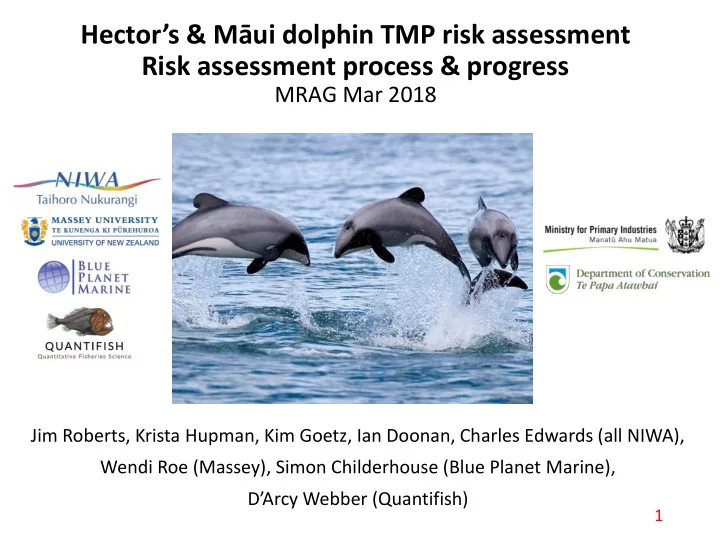
Hectors & Mui dolphin TMP risk assessment Risk assessment process & progress MRAG Mar 2018 Jim Roberts, Krista Hupman, Kim Goetz, Ian Doonan, Charles Edwards (all NIWA), Wendi Roe (Massey), Simon Childerhouse (Blue Planet Marine),
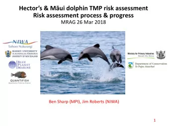
Hector’s & Māui dolphin TMP risk assessment Risk assessment process & progress MRAG Mar 2018 Jim Roberts, Krista Hupman, Kim Goetz, Ian Doonan, Charles Edwards (all NIWA), Wendi Roe (Massey), Simon Childerhouse (Blue Planet Marine), D’Arcy Webber ( Quantifish) 1
Acknowledgements Dolphin experts consulted to date People that have agreed to share data, code & model outputs with the TMP risk assessment… • Darryl MacKenzie & Deanna Clement • Rochelle Constantine & Scott Baker • Jody Weir, Manue Martinez, Stefan Bräger & Sam DuFresne AEWG, MRAG, independent expert reviewers 2
Structure of presentation 1. TMP risk assessment methodology 2. TMP risk assessment process 3. Details & progress with project components 4. What next? 3
Evolution of the Hector’s Māui TMP 2007 TMP M ā ui & Hectors • PBR for 4 genetic sub-populations • Quantitative assessment of set-net mortalities (Davies et al. 2008) • Qualitative assessment of other threats 4
Evolution of the Hector’s M ā ui TMP 2007 TMP M ā ui & Hectors • PBR for 4 genetic sub-populations • Quantitative assessment of set-net mortalities (Davies et al. 2008) • Qualitative assessment of other threats 2012 TMP M ā ui only • PBR for M ā ui • Expert threat characterization – spatial & magnitude (Currey et al. 2012) • Basic assessment of spatial overlap of threats with M ā ui 2017 TMP M ā ui & Hector’s • Spatially-explicit risk assessment (SEFRA) with seasonality • Multiple threats on 4 genetic sub-populations simultaneously • Related to a PST (inspired by though different to PBR approach) 5
TMP risk assessment methodology (1) Extension of SEFRA Risk Atlas tool (Webber: MPI contracts PRO2016096 & SEA2016- 30, in progress), building on initial outputs of the Marine Mammal risk assessment (Dragonfly DataScience: MPI contract PRO2014-01) and method development by Sharp (2017) and Webber & Sharp (in progress) Calculation of Population Suitability Threshold (PST) – annual mortality that will allow population recovery or stabilization to [X] % of K with [Y] certainty, including inter-annual stochasticity 𝑄𝑇𝑈 = 1 2 . 𝜒. 𝑠 𝑛𝑏𝑦 . 𝑂 This will be related to thre at-specific annual potential fatalities (APF) , given overlap between the spatial distribution of Hector’s & Mā ui dolphins and spatial threat intensity The TMP risk assessment will estimate all inputs in blue 6
TMP risk assessment methodology (2) Demographic assessment • Review life history info for Rmax • Current adult survival • Small population-size effects Threat characterisation • Identification of threats • Spatial distribution of threat intensity • Method for estimation of annual threat mortality Hector’s & Mā ui seasonal spatial distribution • Predictive modelling of summer/winter dolphin distribution from aerial surveys (e.g. MacKenzie & Clement 2016) • Integration of info from C-POD, boat-based surveys, etc 7
TMP risk assessment methodology (3 (3) Modifications to SEFRA model • To bring in multiple threats • Population specific demographics • Other custom.. E.g. use of public and/or fishery observer sightings to inform spatial distribution of M ā ui & Hectors Workshop • Review SEFRA model inputs • Implement SEFRA tool • Estimate/illustrate effects of alternative management scenarios on risk • Workshop reporting Risk assessment reporting 8
Māui/Hector’s TMP risk assessment process Project component Sep Oct Nov Dec Jan Feb Mar Apr May Jun Jul Aug Sep Oct Nov Demographic assessment AEWG Threat distributions AEWG Hector’s & Mā ui distributions AEWG Integration into SEFRA Workshop Risk assessment reporting Draft Final 9
Timeline of review opportunities • Aug 2017 – Technical WG, introduction & extending SEFRA for TMP • Sep 2017 – risk assessment begins • Nov 2017 – Toxoplasmosis workshop at Massey • Nov 2017 – AEWG, risk assessment process & progress update • 7 Mar 2018 – AEWG Demographic assessment • 26 Mar 2018 – MRAG, progress update (Auckland) • 17 Apr 2018 – AEWG Threat characterization (MPI, Wellington) • 30 May 2018 – AEWG M ā ui /Hector’s spatial distribution (NIWA, Wellington) • Jul 2018 – SEFRA workshop • Sep/Nov 2018 – TMP risk assessment draft & final reporting 10
Demographic assessment Summary of 7 th March AEWG • Hector’s/Māui rmax (Presented by Charles Edwards) • Small population effect on growth rate ( Ian Doonan ) • Population-specific survival ( Jim Roberts ) 11
Previous Māui TMP r max • 0.018 used as base case by previous TMP (Currey et al. 2012), based on longevity of 20 years… though ~15% survived to age 20+ by 2006… • No updated longevity information is available for this assessment Gormley 2009 Min age in 2006 12
Cetacean r max 𝑠 𝑛𝑏𝑦 = 0.018 is inconsistent with estimates from other mammals given first • reproduction at age 8 (Slooten 1991) • Approx. half the next lowest estimated for a cetacean (Bowhead whales: longevity > 100 years with 𝑠 𝑛𝑏𝑦 ≥ 0.036 ; Givens et al. 2013) 13
Cetacean r max • Direct estimation requires long time series of abundance/demographic rates of populations growing at maximum rate • PBR method the standard risk assessment method in the US (http://www.nmfs.noaa.gov/pr/sars/species.htm). • Default r max of 0.04 is used in 153 of 163 stock assessments due to lack of data; • Of the remainder: • 9 assume r max > 0.04 (e.g. humpback whales) • r max 0.035 is used for one orca population 14
Rmax estimation from Hector’s life history Follows that of Moore (2015) and Dillingham et al (2016) RATIONALE • STEP 1 generates samples for ln(𝜇 𝑛𝑏𝑦 ) consistent with demographic theory • STEP 2 ensures these samples are consistent with allometric theory • These contrasting paradigms are biased in opposite directions by uncertain adult survivorship • Their combined use should intuitively reduce the bias overall 15
Maximum growth rate estimates 16
rmax estimate for Hector’s/Māui 𝑠 𝑛𝑏𝑦 ≈ 0.05 • • Plausible given probable age at first reproduction • Will update with new age data when available 17
Estimating the age at first breeding • An informative prior was developed following a meta-analysis which shows a relationship between asymptotic length and the length at maturity 𝑀 𝛽 ≈ 0.95 𝑀 ∞ 18
Population size bias on pop. growth rate • IBM model population simulations using VORTEX software – simulates demographic stochasticty & Probability Deterministic Stochastic SD Stochastic other low population size extinction Start N rmax rmax rmax (%, within problems 200yr) • Input demographic rates 60 0.04 0.033 0.067 0 consistent with rmax = 0.04 40 0.04 0.031 0.068 0 • Has environmental 35 0.04 0.029 0.069 0 variation & inbreeding 30 0.04 0.028 0.070 0.2 depression 25 0.04 0.026 0.072 2.1 • Realised population growth 20 0.04 0.023 0.075 4.5 lower than input rmax 15 0.04 0.019 0.081 11.4 • 10 0.04 0.011 0.093 36.1 Can be considered for rmax used for Māui 5 0.04 -0.001 0.131 88.3 • Note increased extinction rate below 20 individuals 19
Annual survival Adult survival • A constraint on cumulative mortality • By genetic sub-population (though low info for some e.g. WCSI & SCSI) • Demographic assessment of mark-resighting data using NIWA’s SeaBird • We have or will obtain: o M ā ui genetic & photo mark ID 2001-2017 (from Rochelle & Scott) Progress with M ā ui assessment under DOC project (DOC307002) o Hector’s Kaikoura photo ID 2013 -2017 (from Jody Weir) Will obtain latest years over next few weeks o Hector’s Banks Peninsula photo ID 1985 -2002 (Sam DuFresne thesis) Obtaining similar results to DuFresne (2004) Open demographic assessment presentations… 20
Threat characterisation 21
Which threats will be considered? Threats deemed to affect M ā ui population (Currey et al. 2012)… Indirect effects were bundled into natural mortality & addressed by rmax Shortlist from previous TMP… 22
Which threats will be considered? • Plus key threats affecting Hector’s only from 2007 TMP assessment (if any) • Plus threats not specifically addressed by previous TMPs, e.g.: • Toxoplasmosis • Main cause of death at necropsy – Roe et al. 2013 • Subject of recent workshop held at Massey • Prey availability • Fishing effects deemed influential by 2012 TMP, but not climate • Red cod the main prey – short lived & presumed responsive to SST • Potential future threats, e.g. • Iron sand mining • Changes in spatial extent of threats, e.g. oil & gas 23
Modelling approach varies by threat Approach taken will depend on: • Available information (e.g. spatial threat intensity?) • Whether threat is demonstrably lethal Full SEFRA (estimating deaths within model) • Commercial set net & trawl • Recreational fishing (e.g. using vulnerability from commercial) Partial SEFRA (estimating deaths outside of model) • Other threats known to be lethal & with spatial threat intensity • E.g. toxoplasmosis PBR type approach • Lethal threats for which no spatial threat intensity Will obtain risk ratios for these 24
Recommend
More recommend
Explore More Topics
Stay informed with curated content and fresh updates.
