Heat Flow in Space and Time Time-Stepping Via the Leap Frog - PowerPoint PPT Presentation
Heat Flow in Space and Time Time-Stepping Via the Leap Frog Algorithm Rubin H Landau Sally Haerer, Producer-Director Based on A Survey of Computational Physics by Landau, Pez, & Bordeianu with Support from the National Science Foundation
Heat Flow in Space and Time Time-Stepping Via the Leap Frog Algorithm Rubin H Landau Sally Haerer, Producer-Director Based on A Survey of Computational Physics by Landau, Páez, & Bordeianu with Support from the National Science Foundation Course: Computational Physics II 1 / 1
Problem: How Does a Bar Cool? 100 K Insulated Metallic Bar Touching Ice Aluminum bar, L = 1 m, w along x Insulated along length, ends in ice ( T = 0 C) Initially T = 100 C How does temperature vary in space and time? 2 / 1
The Parabolic Heat Equation (Theory) H = − K ∇ T ( x , t ) (1) Nature: heat flow hot → cold 1 � K = conductivity Q ( t ) = d x C ρ ( x ) T ( x , t ) (2) C = sp heat, ρ = density ∂ T ( x , t ) = K C ρ ∇ 2 T ( x , t ) Q ( t ) = contained heat (3) 2 ∂ t Heat Eqn: ∆ T from flow 3 ∂ 2 T ( x , t ) ∂ T ( x , t ) = K (4) ∂ x 2 ∂ t C ρ Parabolic PDE in x & t 4 400 sin k n x e − α k 2 ∞ n t “Analytic” Solution 5 � T ( x , t ) = (5) n π n = 1 , 3 ,... IC: T ( x , t = 0 ) = 100C ( k n = n π L , α = K C ρ ) (6) BC: T ( x = 0 ) = T ( x = L ) = 0C 3 / 1
Solution Via Time Stepping Differential → difference eqtn x Solve at x − t lattice sites i-1,j i+1,j Vert blue = BC, row 0 = IC t i,j+1 Relax: if knew T bottom Leapfrog ↓ one t to next FD ∂ t , CD for ∂ 2 x (can) ⇒ difference heat eqtn ≃ T ( x , t + ∆ t ) − T ( x , t ) ∂ T ∂ t ∆ t Explicit Soltn : known values ∂ 2 T Not space-time symmetric ≃ T ( x + ∆ x ) + T ( x − ∆ x ) − 2 T ( x ) ∂ x 2 (∆ x ) 2 T ( x , t + ∆ t ) − T ( x , t ) = K T ( x + ∆ x , t ) + T ( x − ∆ x , t ) − 2 T ( x , t ) (1) ∆ t C ρ ∆ x 2 T i , j + 1 = T i , j + η [ T i + 1 , j + T i − 1 , j − 2 T i , j ] (2) 4 / 1
Solution of Heat Equation T 80 0 0 0 10 100 K 40 x t 80 EqHeat.py EqHeat_Animate.py 5 / 1
Von Neumann Stability Analysis T m , j + 1 = T m , j + η [ T m + 1 , j + T m − 1 , j − 2 T m , j ] , x = m ∆ x , t = j ∆ t (1) Assume T m , j = eigenmodes Difference soltn ≃ PDE soltn?? k = 2 π/λ = ? Bad: difference diverges Stable if eigenmodes stable T m , j = ξ ( k ) j e ikm ∆ x (2) i.e. | ξ ( k ) | < 1 ⇒ ξ ( k ) = 1 + 2 η [ cos ( k ∆ x ) − 1 ] (3) Sub (3) into diff eqtn (1) | ξ ( k ) | < 1 (4) ⇒ Smaller ∆ t more stable ⇒ η = K ∆ t C ρ ∆ x 2 < 1 (5) ↓ ∆ x must ↑ ∆ t 2 Always try analysis 6 / 1
Implementation EqHeat.py Build in BC & IC Heart: 2-D array T[101][2] = T[x][present, future] Set future to present, calculate future Output t & T ever 300 t steps Surface T ( x , t ) plots with isotherms , must be smooth Vary ∆ t & ∆ x Compare analytic & numeric solutions Stability: Diverges η > 1 4 ? 7 / 1
Crank–Nicolson Algorithm Next Take a break, or quit if not proceeding to Crank Nicolson. 8 / 1
Recommend
More recommend
Explore More Topics
Stay informed with curated content and fresh updates.


