
Hashing In the last class Implementing Dictionary ADT Definition - PDF document
Algorithm : Design & Analysis [09] Hashing In the last class Implementing Dictionary ADT Definition of red-black tree Black height Insertion into a red-black tree Deletion from a red-black tree Hashing Hashing
Algorithm : Design & Analysis [09] Hashing
In the last class… � Implementing Dictionary ADT � Definition of red-black tree � Black height � Insertion into a red-black tree � Deletion from a red-black tree
Hashing � Hashing � Collision Handling for Hashing � Closed Address Hashing � Open Address Hashing � Hash Functions � Array Doubling and Amortized Analysis
Hashing: the Idea Very large, but only In feasible size a small part is used in an application E[0] • Index distribution E[1] • Collision handling x Hash Key Space Function E[ k ] H ( x )= k Value of a A calculated specific key array index for the key E[ m -1]
Each address is a linked list Collision Handling: Closed Address k 7 k 3 k 4 k 2 k 6 k 1 k 5 k 6 k 5 k 7 k 2 k 4 k 3 k 1
Closed Address: Analysis � Assumption: simple uniform hashing: for j =0,1,2,..., m -1, the average length of the list at E [ j ] is n / m . � The average cost of an unsuccessful search: � Any key that is not in the table is equally likely to hash to any of the m address. The average cost to determine that the key is not in the list E [ h ( k )] is the cost to search to the end of the list, which is n / m . So, the total cost is Θ (1+ n / m ) .
Closed Address: Analysis (cont.) � For successful search: (assuming that x i is the i th element inserted into the table, i =1,2 ,...,n ) � For each i , the probability of that x i is searched is 1/ n . � For a specific x i , the number of elements examined in a successful search is t +1, where t is the number of elements iserted into the same list as x i , after x i has been inserted. And for any j , the probability of that x j is inserted into the same list of x i is 1/ m . So, the cost is: Expected number of ⎛ + ⎞ elements in front of the n n 1 1 ∑ ∑ ⎜ ⎟ searched one in the same 1 ⎜ ⎟ Cost for ⎝ ⎠ n m linked list. computing = = + i 1 j i 1 hashing
Closed Address: Analysis (cont.) � The average cost of a successful search: � Define α =n/m as load factor , The average cost of a successful search is : ⎛ + ⎞ − n n n n 1 ( ) 1 1 1 1 ∑ ∑ ∑ ∑ ⎜ ⎟ = + − = + 1 1 n i 1 i ⎜ ⎟ n ⎝ m ⎠ nm nm = = + = = 1 1 1 1 i j i i i − α α n 1 = + = + − = Θ + α 1 1 ( 1 ) 2 m 2 2 n Number of elements in front of the searched one in the same linked list. Cost for computing hashing
Collision Handling: Open Address � All elements are stored in the hash table, no linked list is used. So, α , the load factor, can not be larger than 1. � Collision is settled by “rehashing”: a function is used to get a new hashing address for each collided address, i.e. the hash table slots are probed successively, until a valid location is found. � The probe sequence can be seen as a permutation of (0,1,2,..., m -1)
Commonly Used Probing Linear probing: Given an ordinary hash function h ’, which is called an auxiliary hash function, the hash function is: (clustering may occur) h ( k , i ) = ( h ’( k )+ i ) mod m ( i =0,1,..., m -1) Quadratic Probing: Given auxiliary function h ’ and nonzero auxiliary constant c 1 and c 2 , the hash function is: (secondary clustering may occur) h ( k , i ) = ( h ’( k )+ c 1 i + c 2 i 2 ) mod m ( i =0,1,..., m -1) Double hashing: Given auxiliary functions h 1 and h 2 , the hash function is: h ( k , i ) = ( h 1 ( k )+ ih 2 ( k )) mod m ( i =0,1,..., m -1)
Linear Probing: an Example H Hash function: h(x)=5x mod 8 Index Hash function: h(x)=5x mod 8 0 1776 1 2 1812 hashing 1055 3 1492 4 1945 rehashing g i n h a s h 5 1812 6 1918 Rehash function: rh(j)=(j+1) mod 8 Rehash function: rh(j)=(j+1) mod 8 7 1945 chain of rehashings
Equally Likely Permutations � Assumption: each key is equally likely to have any of the m ! permutations of (1,2..., m -1) as its probe sequence. � Note: both linear and quadratic probing have only m distinct probe sequence, as determined by the first probe.
Analysis for Open Address Hash � Assuming uniform hashing, the average number of probes in an unsuccessful search is at most 1/(1- α ) ( α = n / m <1) Note : the probabilit y of the first probed position being occupied + n n-j 1 > is , and that of the th( 1 ) position occupied is , j j + m m-j 1 so, the probabilit y of the number of probe no less than i will be : − − − − + i 1 ⎛ ⎞ n n 1 n 2 n i 2 n − ⋅ ⋅ ⋅ ⋅ ≤ = α ⎜ ⎟ i 1 L − − − + ⎝ ⎠ m m 1 m 2 m i 2 m ∞ ∞ 1 ∑ ∑ − α = α = i 1 i Then, the average number of probe is : − α 1 = = i 1 i 0
Analysis for Open Address Hash � Assuming uniform hashing, the average cost of probes in an 1 1 ln ( α = n / m <1) successful search is at most α − α 1 + To search for the ( i 1 ) th inserted element in the table, the cost is the same as the cost for inserting it when th ere i α = are just elements in the table. At that ti me, , so, i m 1 m = For your reference: the cost is For your reference: − i m i 1 - Half full: 1.387; 90% full: 2.559 Half full: 1.387; 90% full: 2.559 m So, the cost is : − − n 1 n 1 m 1 1 1 1 1 1 1 1 ∑ m m ∑ ∑ dx m ∫ m = = ≤ = = ln ln − − α α α − α − α − n m i n m i i x m n 1 m n = = = − + i 0 i 0 i m n 1
Hashing Function � A good hash function satisfies the assumption of simple uniform hashing. � Heuristic hashing functions � The division method: h ( k )= k mod m � The multiplication method: h ( k )= ⎣ m ( kA mod 1) ⎦ (0< A <1) � No single function can avoid the worst case Θ ( n ), so, “Universal hashing” is proposed. � Rich resource about hashing function: Gonnet and Baeza-Yates: Handbook of Algorithms and Data Structures , Addison-Wesley, 1991
Array Doubling � Cost for search in a hash table is Θ (1+ α ), then if we can keep α constant, the cost will be Θ (1) � Space allocation techniques such as array doubling may be needed. � The problem of “unusually expensive” individual operation.
Looking at the Memory Allocation � hashingInsert(HASHTABLE H , ITEM x ) integer size =0, num =0; � if size =0 then allocate a block of size 1; size =1; � if num = size then � Insertion with allocate a block of size 2 size ; � expansion: cost size move all item into new table; � size =2 size ; � insert x into the table; � num = num +1; � Elementary insertion: cost 1 � return
Worst-case Analysis of the Insertion � For n execution of insertion operations � A bad analysis: the worst case for one insertion is the case when expansion is required, up to n � So, the worst case cost is in O ( n 2 ). � Note the expansion is required during the i th operation only if i =2 k , and the cost of the i th operation − ⎧ i if i 1 is exactly power of 2 = ⎨ c i ⎩ 1 otherwise ⎣ ⎦ lg n n ∑ ∑ ≤ + < + = j So, the total cost is : c n 2 n 2 n 3 n i = = i 1 j 0
Amortized Time Analysis � Amortized equation: amortized cost = actual cost + accounting cost � Design goals for accounting cost � In any legal sequence of operations, the sum of the accounting costs is nonnegative. � The amortized cost of each operation is fairly regular, in spite of the wide fluctuate possible for the actual cost of individual operations.
Amortized Analysis: MultiPop Stack Pop: MultiPop: Cost=1 Cost=min( s , t ) Push: Cost=1 s t Amortized cost: push:2; pop, multipop: 0
Amortized Analysis: Binary Counter 0 0 0 0 0 0 0 0 0 0 1 0 0 0 0 0 0 0 1 1 2 0 0 0 0 0 0 1 0 3 Cost measure: bit flip 3 0 0 0 0 0 0 1 1 4 4 0 0 0 0 0 1 0 0 7 5 0 0 0 0 0 1 0 1 8 6 0 0 0 0 0 1 1 0 10 amortized cost: 7 0 0 0 0 0 1 1 1 11 set 1: 2 8 0 0 0 0 1 0 0 0 15 set 0: 0 9 0 0 0 0 1 0 0 1 16 10 0 0 0 0 1 0 1 0 18 11 0 0 0 0 1 0 1 1 19 12 0 0 0 0 1 1 0 0 22 13 0 0 0 0 1 1 0 1 23 14 0 0 0 0 1 1 1 0 25 15 0 0 0 0 1 1 1 1 26 16 0 0 0 1 0 0 0 0 31
Accounting Scheme for Stack Push � Push operation with array doubling � No resize triggered: 1 � Resize( n → 2 n ) triggered: t n +1 (t is a constant) � Accounting scheme (specifying accounting cost) � No resize triggered: 2 t � Resize( n → 2 n ) triggered: - nt +2 t � So, the amortized cost of each individual push operation is 1+2 t ∈Θ (1)
Home Assignment � pp.302- � 6.18 � 6.19 � 6.1 � 6.2
Recommend
![Union-Find [10] In the last class Hashing Collision Handling for Hashing Closed](https://c.sambuz.com/1022731/union-find-s.webp)


More recommend
Explore More Topics
Stay informed with curated content and fresh updates.