Graphical Representation of Causal Effects November 10, 2016 - PowerPoint PPT Presentation
Graphical Representation of Causal Effects November 10, 2016 Lords Paradox: Observed Data Units: Students; Covariates: Sex, September Weight; Potential Outcomes: June Weight under Treatment and Control; Treatment = University diet; Control
Graphical Representation of Causal Effects November 10, 2016
Lord’s Paradox: Observed Data Units: Students; Covariates: Sex, September Weight; Potential Outcomes: June Weight under Treatment and Control; Treatment = University diet; Control = ?? Statistician 1: June weight under control = September weight Statistician 2: June weight under control = a linear function of September weight, i.e. 𝐹[𝑍 0 ] = 𝛾 ( + 𝛾 * 𝑇𝑓𝑦 + 𝛾 . 𝑋𝑓𝑗ℎ𝑢 456 Wainer H and Brown L (2007). Three Statistical Paradoxes in the Interpretation of Group Differences: Illustrated with Medical School Admission and Licsencing Data. Handbook of Statistics .
Assignment Mechanism • Determines which units receive treatment, which receive control • 𝑄 𝑈 𝑌, 𝑍 0 , 𝑍 1 • Known for randomized trials; unknown for observational studies • Model for assignment mechanism necessary (sometimes sufficient) - Model of “science”, 𝑄 𝑍 0 , 𝑍 1 𝑌 not necessary if one knows the assignment mechanism, e.g., randomized trials • So, what’s wrong with the assignment mechanism in Lord’s Paradox?
Key Property of Randomized Trials • Treatment assignment is “unconfounded”, also known as “conditional exchangeability” • 𝑄 𝑈 𝑌, 𝑍 0 , 𝑍 1 = 𝑄 𝑈 𝑌 • Assignment does not depend on potential outcomes • Removes confounding of all variables • Crucial for observational studies, but usually as an unverifiable assumption • Positivity: each unit has a positive probability of receiving each treatment < 1 for all X • 0 < 𝑄 𝑈 𝑌 • Everyone in the study relevant for comparisons • Study must be designed without the use of the knowledge of outcomes Randomization ensures balance of covariates.
Example: Truth vs Observation
Causal Diagram • Directed Acyclic Graph vs Causal Directed Acyclic Graph • Can represent both association and causation • Absence of an arrow from A to Y means no individual in the population has that direct causal effect; Presence of an arrow from A to Y means there is at least one individual in the population having the causal effect • All common causes, even if unmeasured, of any pair of variables on the graph are themselves on the graph • Any Variable is a cause of its descendants
Causal Diagram (continued) • A standard causal diagram does not distinguish whether an arrow represent a harmful effect or protective effect • A variable, if having two causes, the diagram does not encode how the two causes inter
Causal Markov Assumption • Causal DAGs are of no practical use unless we make an assumption linking the causal structure represented by the DAG to the data obtained in a study. We refer to such assumptions as causal Markov assumption : • Conditional on its direct causes, a variable is independent of any variable for which it is not a cause • Equivalent to: conditional on its parents, a node is independent of its non-descendants • Mathematically equivalent to the statement that the density 𝑔(𝑊) of all the variables V in DAG G satisfies the F Markov factorization 𝑔 𝑤 = ∏ 𝑔(𝑤 C ∣ 𝑄𝑏 C ) CG*
Association vs Causation
Causal Diagram for Structural Representation of Biases under the Null • Common causes for treatment A and outcome Y • Common effect for treatment A and outcome Y • Measurement error on the nodes
Assignment Mechanism • Marginal Randomization • Conditional Randomization • Can the above represent observational studies? (Equivelent to assuming conditional exchangeability)
Exchangeability Stratum M=1 • Unconditional Exchangeability • Conditional Exchangeability
Effect Modification and Cancellation of Effects
Effect Modification Under Conditional Randomization or Conditional Exchangeability Stratum M=1
Causal Diagram for Effect Modification (with causal effect on outcome)
Causal Diagram for Effect Modification (without causal effect on outcome)
Alternative Representations • Single World Intervention Graph (SWIG, Richardson and Robins, 2013): seamlessly unifies the counterfactual and graphical approaches to causality by explicitly including the counterfactual variables on the graph • Influence Diagrams . Based on decision theory (Dawid, 2000, 2002). Make no reference to counterfactuals and uses causal diagrams augmented with decision nodes to represent the interventions of interest.
Reading • Hernan and Robins (2016), Chapter 6, Causal Inference. https://www.hsph.harvard.edu/miguel- hernan/causal-inference-book/
Recommend
More recommend
Explore More Topics
Stay informed with curated content and fresh updates.
