Randomized Experiments The goal of randomized experiments is to - PowerPoint PPT Presentation

Randomized Experiments • The goal of randomized experiments is to identify…  The causal effect!  Advantage of causal effect described by statisticians:  “The advantage of causal predictors compared with non-causal predictors is that their influence on the target variable remains invariant under different changes of the environment.” (Peters, Buhlmann and Meinshausen 2016, Journal of the Royal Statistical Society ) • Correlation is not causation!

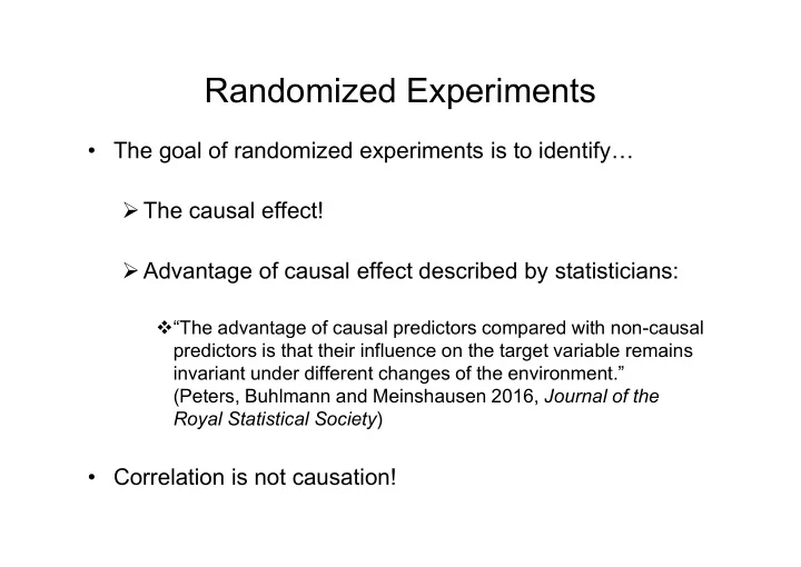
Randomized Experiments • The gold standard to estimate a causal effect is a randomized experiment. • The validity of a randomized experiment depends on: 1. Randomization. 2. Well constructed control group.

What to Take into Account when Conducting a Randomized Experiment? 1) What to randomize on : 1. Randomize eligibility 2. Randomize after acceptance into the program 3. Randomize incentives for take-up Randomize after acceptance into the program: – R=1 if randomized in (treatment group) – R=0 if randomized out (control group) – D denotes if someone applies to the program and is subject to randomization [here D=1 for all people who are in the randomization] – Random assignment implies: • For treatment group: E(Y1|X, D=1,R=1) = E(Y1|X, D=1) • For control group: E(Y0|X, D=1, R=0) = E(Y0|X, D=1)  Experiment gives TTE = E(Y1-Y0|X, D=1)

What to Take into Account when Conducting a Randomized Experiment? 2) Power calculations • Def: power of the design is the probability that, for a given effect size and statistical significance level, we will be able to reject the hypothesis of zero effect. • Design choices that affect the “power” of an experiment: – Sample size – Minimum size of the effect that the researcher wants to be able to detect – Multiple treatment groups – Partial compliance and drop out – Control variables (important to know how much they absorb of the residual variance) • Standard softwares for the single-site case (“power” command in Stata) • Multi-site power analyses get complicated – Need to know the impact variation and correlations across sites

What to Take into Account when Conducting a Randomized Experiment? 3) Choosing the sites in multi-site experiments • External validity: choose sites at random • Realistic impacts: choose sites that are representative • Efficacy: choose sites that will best implement the treatment • Avoid contamination: choose sites with little or no contact of any sort

Examples of Randomized Experiments • Large-scale experiments, e.g. in the US/Canada: – US National JTPA (Job Training Partnership Act) Study, Tennessee class size experiment (STAR) • More recently, randomized experiments in developing countries: – Small experiments addressing very specific questions, for example microfinance experiments by Dean Karlan, education experiments (e.g. schooling inputs) by Michael Kremer and Esther Duflo, etc – Example of a large-scale and very successful conditional cash transfer program: Progresa/Oportunidades in Mexico (1997- 2003)

Example: the STAR Experiment (Stock and Watson Ch. 13) Tennessee Project STAR (Student-Teacher Achievement Ratio):  4-year US study for an overall budget of $12 million. 79 Tennessee public schools for a single cohort of students in kindergarten through third grade in the years 1985-89.  Upon entering the school system a student was randomly assigned to one of three groups:  Regular class (22 – 25 students).  Regular class + full-time teacher’s aide.  Small class (13 – 17 students).  Regular classes’ students re-randomized after first year to regular or regular + aide class.  Y = Stanford achievement test scores.

“Natural” (or Quasi-) Experiments A quasi-experiment or natural experiment : “nature” provides random events that can be used as a source of exogenous variation. Treatment ( D ) is “as if” randomly assigned. Example:  Effect of changes in minimum wage on employment.  D = change in minimum wage law in some States (it changes only in some States, thus State is “as if” randomly assigned). The natural random event operates as an instrumental variable:  Relevance: it is strongly correlated with the treatment D (so much that it defines the treatment!).  Exogeneity: it does not affect the outcome Y rather than via the treatment D .

“Natural” (or Quasi-) Experiments Idea of quasi-experiments follows that of “real” randomized experiments:  find exogenous source of variation (i.e. variable that affects participation but not the outcome directly)  Important to understand the source of variation that helps to identify the treatment effect

“Natural” (or Quasi-) Experiments  Disadvantage: small amount of random events provided by nature…  Advantage: when the nature provides random events, they can usefully be exploited. Example: Card D. and Krueger A. (1994) “Minimum Wages and Employment: A Case Study of the Fast-Food Industry in New Jersey and Pennsylvania”, American Economic Review, Vol. 84, No. 4, pp. 772-793.

Regression Analysis of Experiments for Differences Estimator • In an ideal randomized controlled experiment the treatment D is randomly assigned: Y=a+b*D+u (1) • If D is randomly assigned, then u and D are independently distributed, E(u|D)=0 ( conditional mean independence ) dE(Y|D)/dD=b  average causal effect of D on Y  OLS of (1) gives an unbiased estimate of the causal effect of D on Y. • When the treatment is binary, the causal effect b is the difference in mean outcomes in treatment vs control.  This difference in means is the differences estimator

Regression Analysis of Experiments for Differences Estimator We can add covariates X to the model: Y=a+b*D+c*X+u (2) Advantages of adding the covariates X: 1. Check if randomization worked: if D is randomly assigned, the OLS estimates of b in model (1) and (2) (that is with and without the covariates X) should be similar – if they aren’t, this suggests that D was not randomly assigned • NOTE : to check directly for randomization, we can regress the treatment indicator, D, on the covariates X, and do a F-test. 2. Increases efficiency: smaller standard errors 3. Adjust for conditional randomization (apply conditional randomization if interested in treatment effects for different groups; for example schools’ effects if randomization was within but not across schools).

Problems with Randomized Experiments • Randomization per se does not assure that the treatment and the control group are perfectly comparable. – In any given RCT, nothing ensures that other causal factors are balanced across the groups at the point of randomization (Deaton and Cartwright 2017). • Randomization per se only means that, on average, if several experiments are repeated, the estimated effect of the treatment is the true effect. – Unbiasedness says that, if we were to repeat the trial many times, we would be right on average. Yet we are almost never in such a situation, and with only one trial (as is virtually always the case) unbiasedness does nothing to prevent our single estimate from being very far away from the truth (Deaton and Cartwright 2017).

Solvable Problems with Randomized Experiments 1. Drop-out of treatment: some subjects in the treatment group may drop out before completing the program. 2. Contamination bias: some subjects in the control group get treatment.

Two Solutions to Drop-out of Treatment and Contamination Bias 1. Define treatment as “intent-to-treat” or “offer of treatment”: focus on those who were invited to be treated, whether or not they actually agreed to be treated. 2. Treatment assignment can be used as an instrument: • Wald estimator: IV when the instrument is a binary variable.

Wald Estimator to Solve Drop-out of Treatment and Contamination Bias Start with some notation: – Initial random assignment: R=0/1 – Decision to participate: D=0/1 Drop out of treatment: R=1 and D=0   Contamination bias: R=0 and D=1 p0=P(D=1|R=0), p1=P(D=1|R=1) Observe R, D, p0, p1, Y0 if D=0 and Y1 if D=1   E(Y|R=0)=E(Y1|R=0)*p0 + E(Y0|R=0)*(1-p0) E(Y|R=1)=E(Y1|R=1)*p1 + E(Y0|R=1)*(1-p1)

Wald Estimator to Solve Drop-out of Treatment and Contamination Bias Given: E(Y|R=0)=E(Y1|R=0)*p0 + E(Y0|R=0)*(1-p0) E(Y|R=1)=E(Y1|R=1)*p1 + E(Y0|R=1)*(1-p1) Because of Randomization: E(Y1|R=1)=E(Y1|R=0)=E(Y1) (same for Y0) Therefore: E(Y|R=1) – E(Y|R=0)= E(Y1)*(p1-p0) – E(Y0)*(p1-p0)  ATE= E(Y1) – E(Y0)= [E(Y|R=1)-E(Y|R=0)]/(p1-p0) [Wald estimator]

Unsolvable Problems with Randomized Experiments • Not implementable: e.g. effect of a merger on a firm’s outputs – we can not force a firm to merge. • Costs are too high. • Ethical considerations: e.g. all poor households should receive a given income subsidy. • Estimates would only be available after many years: e.g. effect of healthy diet on longevity.