Graphical models and inference II Milos Hauskrecht milos@pitt.edu - PDF document

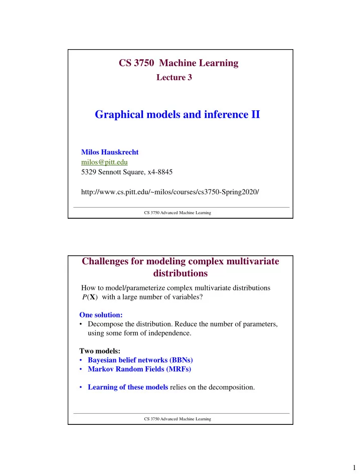
CS 3750 Machine Learning Lecture 3 Graphical models and inference II Milos Hauskrecht milos@pitt.edu 5329 Sennott Square, x4-8845 http://www.cs.pitt.edu/~milos/courses/cs3750-Spring2020/ CS 3750 Advanced Machine Learning Challenges for modeling complex multivariate distributions How to model/parameterize complex multivariate distributions ( X ) with a large number of variables? P One solution: • Decompose the distribution. Reduce the number of parameters, using some form of independence. Two models: • Bayesian belief networks (BBNs) • Markov Random Fields (MRFs) • Learning of these models relies on the decomposition. CS 3750 Advanced Machine Learning 1

Bayesian belief network Directed acyclic graph • Nodes = random variables • Links = direct (causal) dependencies Missing links encode different marginal and conditional independences P (B) P (E) Burglary Earthquake Alarm P (A|B,E) P (M|A) P (J|A) MaryCalls JohnCalls CS 3750 Advanced Machine Learning Bayesian belief network P (B) P (E) T F T F Burglary 0.001 0.999 Earthquake 0.002 0.998 P (A|B,E) B E T F T T 0.95 0.05 T F 0.94 0.06 Alarm F T 0.29 0.71 F F 0.001 0.999 P (J|A) P (M|A) A T F A T F T 0.90 0.1 JohnCalls MaryCalls T 0.7 0.3 F 0.05 0.95 F 0.01 0.99 CS 3750 Advanced Machine Learning 2

Full joint distribution in BBNs The full joint distribution is defined as a product of local conditional distributions:   P ( , ,.., ) P ( | ( ) ) X X X X pa X 1 2 n i i  1 ,.. i n B E Example: A Assume the following assignment of values to random variables M      J , , , , B T E T A T J T M F Then its probability is:       P ( B T , E T , A T , J T , M F )          ( ) ( ) ( | , ) ( | ) ( | ) P B T P E T P A T B T E T P J T A T P M F A T CS 3750 Advanced Machine Learning Inference in Bayesian networks • Full joint uses the decomposition • Calculation of marginals: – Requires summation over variables we want to take out B E   ( ) P J T A           ( , , , , ) P B b E e A a J T M m J M     , , , , b T F e T F a T F m T F • How to compute sums and products more efficiently?    ( ) ( ) af x a f x x x 3

Variable elimination  Assume order: M, E, B, A to calculate ( ) P J T               ( | ) ( | ) ( | , ) ( ) ( ) P J T A a P M m A a P A a B b E e P B b P E e     , , , , b T F e T F a T F m T F                 ( | ) ( | , ) ( ) ( )  ( | )  P J T A a P A a B b E e P B b P E e P M m A a       , , , , b T F e T F a T F m T F            ( | ) ( | , ) ( ) ( ) 1 P J T A a P A a B b E e P B b P E e    , , , b T F e T F a T F              ( | ) ( )  ( | , ) ( )  P J T A a P B b P A a B b E e P E e      , , , a T F b T F e T F          ( | ) ( ) ( , ) P J T A a P B b A a B b 1   , , a T F b T F            ( | )  ( ) ( , )  P J T A a P B b A a B b 1     , , a T F e T F         ( | ) ( ) ( ) P J T A a A a P J T 2  a T , F Variable elimination  Assume order: M, E, B, A to calculate ( ) P J T               P ( J T | A a ) P ( M m | A a ) P ( A a | B b , E e ) P ( B b ) P ( E e )     , , , , b T F e T F a T F m T F      ( ) ( , ) ( , , ) ( ) ( ) f A f M A f A B E f B f E 1 2 3 4 4     , , , , B T F E T F A T F M T F Conditional probabilities defining the joint = factors Variable elimination inference can be cast in terms of operations defined over factors 4

Factors • Factor: is a function that maps value assignments for a subset of random variables to  (reals) • The scope of the factor: – a set of variables defining the factor • Example: – Assume discrete random variables x (with values a1,a2, a3) and y (with values b1 and b2) – Factor: a1 b1 0.5 a1 b2 0.2  ( , ) x y a2 b1 0.1 – Scope of the factor: a2 b2 0.3 { , } x y a3 b1 0.2 a3 b2 0.4 CS 3750 Advanced Machine Learning Factor Product Variables: A,B,C      ( A , B , C ) ( B , C ) ( A , B )  ( A , B , C )   ( A , B ) a1 b1 c1 0.5*0.1 ( B , C ) a1 b1 c2 0.5*0.6 a1 b2 c1 0.2*0.3 a1 b1 0.5 a1 b2 c2 0.2*0.4 b1 c1 0.1 a1 b2 0.2 a2 b1 c1 0.1*0.1 b1 c2 0.6 a2 b1 c2 0.1*0.6 a2 b1 0.1 a2 b2 c1 0.3*0.3 b2 c1 0.3 a2 b2 0.3 a2 b2 c2 0.3*0.4 a3 b1 c1 0.2*0.1 b2 c2 0.4 a3 b1 0.2 a3 b1 c2 0.2*0.6 a3 b2 0.4 a3 b2 c1 0.4*0.3 a3 b2 c2 0.4*0.4 CS 3750 Advanced Machine Learning 5

Factor Marginalization     Variables: A,B,C ( , ) ( , , ) A C A B C B a1 b1 c1 0.2 a1 b1 c2 0.35 a1 b2 c1 0.4 a1 b2 c2 0.15 a1 c1 0.2+0.4=0.6 a2 b1 c1 0.5 a1 c2 0.35+0.15=0.5 a2 b1 c2 0.1 a2 c1 0.8 a2 c2 0.3 a2 b2 c1 0.3 a3 c1 0.4 a2 b2 c2 0.2 a3 c2 0.7 a3 b1 c1 0.25 a3 b1 c2 0.45 a3 b2 c1 0.15 a3 b2 c2 0.25 CS 3750 Advanced Machine Learning Factor division A=1 B=1 0.5 A=1 B=1 0.5/0.4=1.25 A=1 B=2 0.4 A=1 B=2 0.4/0.4=1.0 A=1 0.4 A=2 B=1 0.8 A=2 B=1 0.8/0.4=2.0 A=2 0.4 A=2 B=2 0.2 A=2 B=2 0.2/0.4=2.0 A=3 0.5 A=3 B=1 0.6 A=3 B=1 0.6/0.5=1.2 A=3 B=2 0.5 A=3 B=2 0.5/0.5=1.0 Inverse of a factor product CS 3750 Advanced Machine Learning 6

Markov random fields An undirected network (also called independence graph) • Probabilistic models with symmetric dependences • G = (S, E) – S set of random variables – Undirected edges E that define dependences between pairs of variables Example: A G variables A,B ..H H C B F E D CS 3750 Advanced Machine Learning Markov random fields The full joint of the MRF is defined    ( x ) ( x ) P c c  ( ) c cl x  c x ( ) - A potential function (defined over variables in cliques/factors) c A G Example: H C B F Full joint: E D       ( , ,... ) ~ ( , , ) ( , , ) ( , ) ( , ) ( , ) ( , ) P A B H A B C B D E A G C F G H F H 1 2 3 4 5 6  c x ( ) - A potential function (defined over a clique of the graph) c CS 3750 Advanced Machine Learning 7

Markov random fields: independence relations • Pairwise Markov property – Two nodes in the network that are not directly connected can be made independent given all other nodes • Local Markov property – A set of nodes (variables) can be made independent from the rest of nodes variables given its immediate neighbors • Global Markov property – A vertex set A is independent of the vertex set B (A and B are disjoint) given set C if all chains in between elements in A and B intersect C CS 3750 Advanced Machine Learning MRF variable elimination inference A G Example: H A   C P ( B ) P ( A , B ,... H ) B F , C , D ,.. H E D 1         ( , , ) ( , , ) ( , ) ( , ) ( , ) ( , ) A B C B D E A G C F G H F H 1 2 3 4 5 6 Z A , C , D ,.. H A G H C Eliminate E B F E D   1          ( , , ) ( , , ) ( , ) ( , ) ( , ) ( , ) A B C  B D E  A G C F G H F H 1 2 3 4 5 6   Z A , C , D , F , G , H E  ( , ) B D 1 CS 3750 Advanced Machine Learning 8