Graphical models Why All probabilistic inference and learning - PDF document

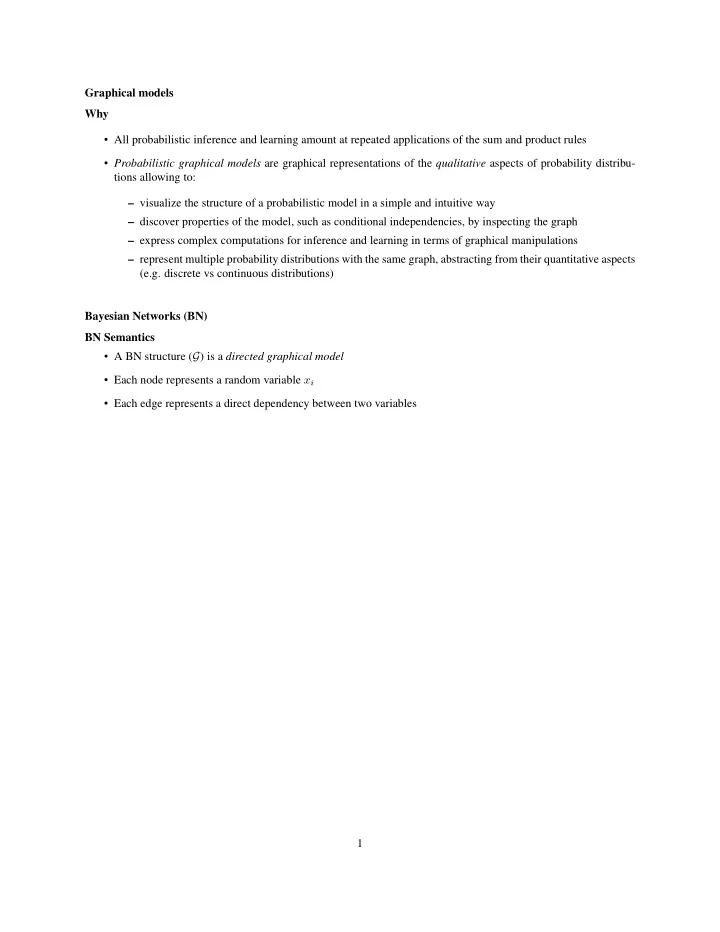
Graphical models Why • All probabilistic inference and learning amount at repeated applications of the sum and product rules • Probabilistic graphical models are graphical representations of the qualitative aspects of probability distribu- tions allowing to: – visualize the structure of a probabilistic model in a simple and intuitive way – discover properties of the model, such as conditional independencies, by inspecting the graph – express complex computations for inference and learning in terms of graphical manipulations – represent multiple probability distributions with the same graph, abstracting from their quantitative aspects (e.g. discrete vs continuous distributions) Bayesian Networks (BN) BN Semantics • A BN structure ( G ) is a directed graphical model • Each node represents a random variable x i • Each edge represents a direct dependency between two variables 1

x 1 x 2 x 3 x 4 x 5 x 6 x 7 The structure encodes these independence assumptions: I ℓ ( G ) = {∀ i x i ⊥ NonDescendants x i | Parents x i } 2

each variable is independent of its non-descendants given its parents Bayesian Networks Graphs and Distributions • Let p be a joint distribution over variables X • Let I ( p ) be the set of independence assertions holding in p • G in as independency map (I-map) for p if p satisfies the local independences in G : I ℓ ( G ) ⊆ I ( p ) 3

x 1 x 2 x 3 x 4 x 5 x 6 x 7 Note The reverse is not necessarily true: there can be independences in p that are not modelled by G . 4

Bayesian Networks Factorization • We say that p factorizes according to G if: m � p ( x 1 , . . . , x m ) = p ( x i | Pa x i ) i =1 • If G is an I-map for p , then p factorizes according to G • If p factorizes according to G , then G is an I-map for p 5

x 1 x 2 x 3 x 4 x 5 x 6 x 7 Example 6

p ( x 1 , . . . , x 7 ) = p ( x 1 ) p ( x 2 ) p ( x 3 ) p ( x 4 | x 1 , x 2 , x 3 ) p ( x 5 | x 1 , x 3 ) p ( x 6 | x 4 ) p ( x 7 | x 4 , x 5 ) Bayesian Networks Proof: I-map ⇒ factorization 1. If G is an I-map for p , then p satisfies (at least) these (local) independences: {∀ i x i ⊥ NonDescendants x i | Parents x i } 2. Let us order variables in a topological order relative to G , i.e.: x i → x j ⇒ i < j 3. Let us decompose the joint probability using the chain rule as: m � p ( x 1 , . . . , x m ) = p ( x i | x 1 , . . . , x i − 1 ) i =1 4. Local independences imply that for each x i : p ( x i | x 1 , . . . , x i − 1 ) = p ( x i | Pa x i ) Bayesian Networks Proof: factorization ⇒ I-map 1. If p factorizes according to G , the joint probability can be written as: m � p ( x i | Pa x i ) p ( x 1 , . . . , x m ) = i =1 2. Let us consider the last variable x m (repeat steps for the other variables). By the product and sum rules: p ( x 1 , . . . , x m ) p ( x 1 , . . . , x m ) p ( x m | x 1 , . . . , x m − 1 ) = p ( x 1 , . . . , x m − 1 ) = � x m p ( x 1 , . . . , x m ) 3. Applying factorization and isolating the only term containing x m we get: � m − 1 ✭ � m p ( x m | Pa x m ) ✭✭✭✭✭✭✭ i =1 p ( x i | Pa x i ) i =1 p ( x i | Pa x i ) = i =1 p ( x i | Pa x i ) = � m ✿ 1 � ✘ ✘✘✘✘✘✘✘✘ x m ✭ ✭✭✭✭✭✭✭ � m − 1 i =1 p ( x i | Pa x i ) � x m p ( x m | Pa x m ) Bayesian Networks Definition A Bayesian Network is a pair ( G , p ) where p factorizes over G and it is represented as a set of conditional probability distributions (cpd) associated with the nodes of G . Factorized Probability m � p ( x i | Pa x i ) p ( x 1 , . . . , x m ) = i =1 7

Bayesian Networks Example: toy regulatory network • Genes A and B have independent prior probabilities • Gene C can be enhanced by both A and B gene value P(value) A 0.3 active A inactive 0.7 gene value P(value) B active 0.3 B inactive 0.7 A active inactive B B active inactive active inactive C active 0.9 0.6 0.7 0.1 C inactive 0.1 0.4 0.3 0.9 Conditional independence Introduction • Two variables a, b are conditionally independent (written a ⊥ b | ∅ ) if: p ( a, b ) = p ( a ) p ( b ) • Two variables a, b are conditionally independent given c (written a ⊥ b | c ) if: p ( a, b | c ) = p ( a | c ) p ( b | c ) 8

• Independence assumptions can be verified by repeated applications of sum and product rules • Graphical models allow to directly verify them through the d-separation criterion d-separation Tail-to-tail • Joint distribution: p ( a, b, c ) = p ( a | c ) p ( b | c ) p ( c ) • a and b are not conditionally independent (written a ⊤ ⊤ b | ∅ ): � p ( a, b ) = p ( a | c ) p ( b | c ) p ( c ) � = p ( a ) p ( b ) c c a b • a and b are conditionally independent given c : p ( a, b | c ) = p ( a, b, c ) = p ( a | c ) p ( b | c ) p ( c ) 9

c a b • c is tail-to-tail wrt to the path a → b as it is connected to the tails of the two arrows d-separation Head-to-tail • Joint distribution: p ( a, b, c ) = p ( b | c ) p ( c | a ) p ( a ) = p ( b | c ) p ( a | c ) p ( c ) • a and b are not conditionally independent : � p ( b | c ) p ( c | a ) � = p ( a ) p ( b ) p ( a, b ) = p ( a ) c a c b • a and b are conditionally independent given c : p ( a, b | c ) = p ( b | c ) p ( a | c ) p ( c ) = p ( b | c ) p ( a | c ) p ( c ) 10

a c b • c is head-to-tail wrt to the path a → b as it is connected to the head of an arrow and to the tail of the other one d-separation Head-to-head • Joint distribution: p ( a, b, c ) = p ( c | a, b ) p ( a ) p ( b ) • a and b are conditionally independent : � p ( a, b ) = p ( c | a, b ) p ( a ) p ( b ) = p ( a ) p ( b ) c a b c • a and b are not conditionally independent given c : p ( a, b | c ) = p ( c | a, b ) p ( a ) p ( b ) � = p ( a | c ) p ( b | c ) p ( c ) 11

a b c • c is head-to-head wrt to the path a → b as it is connected to the heads of the two arrows d-separation General Head-to-head • Let a descendant of a node x be any node which can be reached from x with a path following the direction of the arrows • A head-to-head node c unblocks the dependency path between its parents if either itself or any of its descendants receives evidence Example of head-to-head connection Setting • A fuel system in a car: battery B , either charged ( B = 1 ) or flat ( B = 0 ) fuel tank F , either full ( F = 1 ) or empty ( F = 0 ) electric fuel gauge G , either full ( G = 1 ) or empty ( G = 0 ) Conditional probability tables (CPT) • Battery and tank have independent prior probabilities: P ( B = 1) = 0 . 9 P ( F = 1) = 0 . 9 12

• The fuel gauge is conditioned on both (unreliable!): B F G P ( G = 1 | B = 1 , F = 1) = 0 . 8 P ( G = 1 | B = 1 , F = 0) = 0 . 2 P ( G = 1 | B = 0 , F = 1) = 0 . 2 P ( G = 1 | B = 0 , F = 0) = 0 . 1 Example of head-to-head connection Probability of empty tank • Prior: P ( F = 0) = 1 − P ( F = 1) = 0 . 1 • Posterior after observing empty fuel gauge: 13

B F G P ( F = 0 | G = 0) = P ( G = 0 | F = 0) P ( F = 0) ≃ 0 . 257 P ( G = 0) Note The probability that the tank is empty increases from observing that the fuel gauge reads empty (not as much as expected because of strong prior and unreliable gauge) Example of head-to-head connection Derivation � P ( G = 0 | F = 0) = P ( G = 0 , B | F = 0) B ∈{ 0 , 1 } � = P ( G = 0 | B, F = 0) P ( B | F = 0) B ∈{ 0 , 1 } � = P ( G = 0 | B, F = 0) P ( B ) = 0 . 81 B ∈{ 0 , 1 } � � P ( G = 0) = P ( G = 0 , B, F ) B ∈{ 0 , 1 } F ∈{ 0 , 1 } � � = P ( G = 0 | B, F ) P ( B ) P ( F ) B ∈{ 0 , 1 } F ∈{ 0 , 1 } 14

Example of head-to-head connection Probability of empty tank • Posterior after observing that the battery is also flat: P ( F = 0 | G = 0 , B = 0) = B F G P ( G = 0 | F = 0 , B = 0) P ( F = 0 | B = 0) ≃ 0 . 111 P ( G = 0 | B = 0) Note • The probability that the tank is empty decreases after observing that the battery is also flat • The battery condition explains away the observation that the fuel gauge reads empty • The probability is still greater than the prior one, because the fuel gauge observation still gives some evidence in favour of an empty tank General d-separation criterion d-separation definition • Given a generic Bayesian network • Given A, B, C arbitrary nonintersecting sets of nodes • The sets A and B are d-separated by C ( dsep ( A ; B | C ) ) if: – All paths from any node in A to any node in B are blocked 15

• A path is blocked if it includes at least one node s.t. either: – the arrows on the path meet tail-to-tail or head-to-tail at the node and it is in C , or – the arrows on the path meet head-to-head at the node and neither it nor any of its descendants is in C d-separation implies conditional independence The sets A and B are independent given C ( A ⊥ B | C ) if they are d-separated by C . Example of general d-separation a ⊤ ⊤ b | c • Nodes a and b are not d-separated by c : – Node f is tail-to-tail and not observed – Node e is head-to-head and its child c is observed f a e b c a ⊥ b | f • Nodes a and b are d-separated by f : – Node f is tail-to-tail and observed 16