Graph distance distribution for social network mining Plan of the - PowerPoint PPT Presentation
Graph distance distribution for social network mining Plan of the talk Computing distances in large graphs ( using HyperBall ) Running HyperBall on Facebook ( the largest Milgram - like experiment ever performed ) Other uses of
Graph distance distribution for social network mining
Plan of the talk • Computing distances in large graphs ( using HyperBall )� • Running HyperBall on Facebook ( the largest Milgram - like experiment ever performed )� • Other uses of distances ( in particular: robustness )
Prelude Milgram’s experiment is 45
Where it all started... • M. Kochen, I. de Sola Pool: Contacts and influences. ( Manuscript, early 50s )� • A. Rapoport, W .J. Horvath: A study of a large sociogram . ( Behav.Sci. 1961 )� • S. Milgram, An experimental study of the sma lm world problem. ( Sociometry, 1969 )
Milgram’s experiment • 300 people ( starting population ) are asked to dispatch a parcel to a single individual ( target )� • The target was a Boston stockbroker � • The starting population is selected as follows: � • 100 were random Boston inhabitants ( group A )� • 100 were random Nebraska strockbrokers ( group B )� • 100 were random Nebraska inhabitants ( group C )
Milgram’s experiment • Rules of the game: � • parcels could be directly sent only to someone the sender knows personally � • 453 intermediaries happened to be involved in the experiments ( besides the starting population and the target )
Milgram’s experiment • Questions Milgram wanted to answer: � • How many parcels will reach the target? � • What is the distribution of the number of hops required to reach the target? � • Is this distribution di ff erent for the three starting subpopulations?
Milgram’s experiment • Answers: � • How many parcels will reach the target? 29 % � • What is the distribution of the number of hops required to reach the target? Avg. was 5.2 � • Is this distribution di ff erent for the three starting subpopulations? Y es: avg. for groups A/B/C was 4.6/5.4/5.7, respectively
Chain lengths
Milgram’s popularity • Six degrees of separation slipped away from the scientific niche to enter the world of popular immagination: � • “Six degrees of separation” is a play by John Guare... � • ...a movie by Fred Schepisi... � • ...a song sung by dolls in their national costume at Disneyland in a heart - warming exhibition celebrating the connectedness of people all
Milgram’s criticisms • “Could it be a big world after all? ( The six - degrees - of - separation myth ) ” ( Judith S. Kleinfeld, 2002 )� • The vast majority of chains were never completed � • Extremely di ffi cult to reproduce
Measuring what? • But what did Milgram’s experiment reveal, after all? � i ) That the world is small � ii ) That people are able to exploit this smallness
HyperBall A tool to compute distances in large graphs
Introduction • Y ou want to study the properties of a huge graph ( typically: a social network )� • Y ou want to obtain some information about its global structure ( not simply triangle - counting/degree distribution/etc. )� • A natural candidate: distance distribution
Graph distances and distribution • Given a graph, d ( x,y ) is the length of the shortest path from x to y (∞ if one cannot go from x to y )� • For undirected graphs, d ( x,y ) =d ( y,x )� • For every t , count the number of pairs ( x,y ) such that d ( x,y ) =t � • The fraction of pairs at distance t is ( the density function of ) a distribution
Exact computation • How can one compute the distance distribution? � • W eighted graphs: Dijkstra ( single - source: O ( n 2 )) , Floyd - W arshall ( all - pairs: O ( n 3 )) � • In the unweighted case: � • a single BFS solves the single - source version of the problem: O ( m )� • if we repeat it from every source: O ( nm )
Sampling pairs • Sample at random pairs of nodes ( x,y ) � • Compute d ( x,y ) with a BFS from x � • ( Possibly: reject the pair if d ( x,y ) is infinite )
Sampling pairs • For every t , the fraction of sampled pairs that were found at distance t are an estimator of the value of the probability mass function � • Takes a BFS for every pair O ( m )
Sampling sources • Sample at random a source x � • Compute a full BFS from x
Sampling sources • It is an unbiased estimator only for undirected and connected graphs � • Uses anyway BFS... � • ...not cache friendly � • ...not compression friendly
Cohen’s sampling • Edith Cohen [ JCSS 1997 ] came out with a very general framework for size estimation: powerful, but doesn’t scale well, it is not easily parallelizable, requires direct access
Alternative: Di ff usion • Basic idea: Palmer et. al , KDD ’02 � • Let B t ( x ) be the ball of radius t about x ( the set of nodes at distance ≤ t from x )� • Clearly B 0 ( x ) = { x }� • Moreover B t +1 ( x ) = ∪ x → y B t ( y ) ∪ { x }� • So computing B t +1 starting from B t one just need a single ( sequential ) scan of the graph
A round of updates ☺ ☺ ☺ ☺ ☺ ☺ ☺ ☺ ☺ ☺ ☺ ☺ ☺ ☺ ☺ ☺ ☺ ☺ ☺ ☺
Another round... ☺☺ ☺☺ ☺ ☺ ☺ ☺ ☺ ☺ ☺ ☺ ☺☺ ☺☺ ☺ ☺ ☺ ☺ ☺ ☺ ☺ ☺ ☺ ☺ ☺ ☺ ☺ ☺ ☺ ☺ ☺ ☺
Easy but costly • Every set requires O ( n ) bits, hence O ( n 2 ) bits overall � • Too many! � • What about using approximated sets ? � • W e need probabilistic counters , with just two primitives: add and size? � • V ery small!
HyperBall • W e used HyperLogLog counters [ Flajolet et al. , 2007 ]� • With 40 bits you can count up to 4 billion with a standard deviation of 6 %� • Remember: one set per node!
Observe that • Every single counter has a guaranteed relative standard deviation ( depending only on the number of registers per counter )� • This implies a guarantee on the summation of the counters � • This gives in turn precision bounds on the estimated distribution with respect to the real one
Other tricks • W e use broadword programming to compute e ffi ciently unions � • Systolic computation for on - demand updates of counters � • Exploited micropara lm elization of multicore architectures
Footprint • Scalability: a minimum of 20 bytes per node � • On a 2TiB machine, 100 billion nodes � • Graph structure is accessed by memory - mapping in a compressed form ( W ebGraph )� • Pointer to the graph are store using succinct lists ( Elias - Fano representation )
Performance • On a 177K nodes / 2B arcs graph � • Hadoop: 2875s per iteration [ Kang, Papadimitriou, Sun and H. Tong, 2011 ]� • HyperBall on this laptop: 70s per iteration � • On a 32 - core workstation: 23s per iteration � • On ClueW eb09 ( 4.8G nodes, 8G arcs ) on a 40 - core workstation: 141m ( avg. 40s per iteration )
T ry it! • HyperBall is available within the webgraph package � • Download it from � • http://webgraph.di.unimi.it/ � • Or google for webgraph
Running it on Facebook! [ with Sebastiano Vigna, Marco Rosa, Lars Backstrom and Johan Ugander ]
Facebook • Facebook opened up to non - college students on September 26, 2006 � • So, between 1 Jan 2007 and 1 Jan 2008 the number of users exploded
Experiments ( time ) • W e ran our experiments on snapshots of facebook � • Jan 1, 2007 � • Jan 1, 2008 ... � • Jan 1, 2011 � • [ current ] May, 2011
Experiments ( dataset ) • W e considered: � • fc : the whole facebook � • it / se: only Italian / Swedish users � • it+se: only Italian & Swedish users � • us: only US users � • Based on users’ current geo - IP location
Active users • W e only considered active users ( users who have done some activity in the 28 days preceding 9 Jun 2011 )� • So we are not considering “old” users that are not active any more � • For fc [ current ] we have about 750M nodes
Distance distribution (fc) fb current fb 2008 fb 2007 fb 2010 fb 2009 fb 2011 0.7 0.7 0.7 0.7 0.7 0.7 0.6 0.6 0.6 0.6 0.6 0.6 ● ● ● 0.5 0.5 0.5 0.5 0.5 0.5 ● ● ● 0.4 0.4 0.4 0.4 0.4 0.4 % pairs % pairs % pairs % pairs % pairs % pairs ● 0.3 0.3 0.3 0.3 0.3 0.3 ● ● ● ● ● 0.2 0.2 0.2 0.2 0.2 0.2 ● ● ● ● 0.1 0.1 0.1 0.1 0.1 0.1 ● ● ● ● ● ● ● ● ● 0.0 0.0 0.0 0.0 0.0 0.0 ● ● ● ● ● ● ● ● ● ● ● ● ● ● ● ● ● ● ● ● ● ● ● ● ● ● ● ● ● ● ● ● ● ● ● ● ● ● ● ● ● ● ● ● ● ● ● ● ● ● ● ● ● ● ● ● ● ● ● ● ● ● ● ● ● ● ● ● ● ● ● ● ● ● ● ● ● ● ● ● ● ● ● ● ● ● ● ● ● ● ● ● ● ● ● 0 0 0 0 0 0 5 5 5 5 5 5 10 10 10 10 10 10 15 15 15 15 15 15 distance distance distance distance distance distance
Recommend
More recommend
Explore More Topics
Stay informed with curated content and fresh updates.
