Graph-based Proximity Measures Nagiza F. Samatova William Hendrix - PowerPoint PPT Presentation
Practical Graph Mining with R Graph-based Proximity Measures Nagiza F. Samatova William Hendrix John Jenkins Kanchana Padmanabhan Arpan Chakraborty Department of Computer Science North Carolina State University Outline Defining
Practical Graph Mining with R Graph-based Proximity Measures Nagiza F. Samatova William Hendrix John Jenkins Kanchana Padmanabhan Arpan Chakraborty Department of Computer Science North Carolina State University
Outline • Defining Proximity Measures • Neumann Kernels • Shared Nearest Neighbor 2
Similarity and Dissimilarity • Similarity – Numerical measure of how alike two data objects are. – Is higher when objects are more alike. – Often falls in the range [0,1]: – Examples: Cosine, Jaccard, Tanimoto, • Dissimilarity – Numerical measure of how different two data objects are – Lower when objects are more alike – Minimum dissimilarity is often 0 – Upper limit varies • Proximity refers to a similarity or dissimilarity Src: “Introduction to Data Mining” by Vipin Kumar et al 3
Distance Metric Distance d (p, q) between two points p and q is a • dissimilarity measure if it satisfies: 1. Positive definiteness: d (p, q) ≥ 0 for all p and q and d (p, q) = 0 only if p = q . 2. Symmetry: d (p, q) = d (q, p) for all p and q . 3. Triangle Inequality: d (p, r) ≤ d (p, q) + d (q, r) for all points p , q , and r . Examples: • – Euclidean distance – Minkowski distance – Mahalanobis distance Src: “Introduction to Data Mining” by Vipin Kumar et al 4
Is this a distance metric? ( , ,...., ) and ( , ,...., ) = ∈ d = ∈ d p p p p q q q q � � 1 2 1 2 d d ( , ) max( , ) = d p q p q Not: Positive definite j j 1 ≤ ≤ j d Not: Symmetric ( , ) max( ) = − d p q p q j j 1 ≤ ≤ j d Not: Triangle Inequality d ( , ) ( ) 2 = − d p q p q ∑ j j = 1 j Distance Metric ( , ) min | | = − d p q p q j j 1 ≤ ≤ j d 5
Distance: Euclidean, Minkowski, Mahalanobis ( , ,...., ) and ( , ,...., ) = ∈ d = ∈ d p p p p q q q q � � 1 2 1 2 d d Minkowski Mahalanobis Euclidean ( , ) ( ) − 1 ( ) T 1 = − Σ − d p q p q p q d ( , ) ( ) 2 = − d d p q p q r ( , ) | | = − r ∑ d p q p q j j 1 = ∑ j r j j = 1 j 1: = r City block distance Manhattan distance -norm L 1 2: = r Euclidean, -norm L 2 6
d ( , ) ( ) 2 = − d p q p q Euclidean Distance ∑ j j 1 = j Standardization is necessary, if scales differ. ( , ) = p age salary ( , ,...., ) = ∈ � d p p p p Ex: 1 2 d Standard deviation of attributes Mean of attributes 1 d 1 d = ∈ p p � ( ) 2 = − ∈ s p p ∑ k d � − ∑ p k 1 1 d k = 1 = k Standardized/Normalized Vector 0 = p − − − − p p p p p p p p new ( , ,..., ) = = ∈ � d p 1 2 d 1 = new s s s s s p p p p p new 7
d ( , ) ( ) 2 = − d p q p q Distance Matrix ∑ j j 1 = j • P = as.matrix (read.table(file=“points.dat”)); • D = dist (P[, 2;3], method = "euclidean "); • L1 = dist (P[, 2;3], method = “minkowski " , p=1 ); • help (dist) 3 Input Data Table: P point x y p1 2 p1 0 2 p3 p4 2 0 p2 1 p3 3 1 p2 p4 5 1 0 0 1 2 3 4 5 6 File name: points.dat Output Distance Matrix : D p1 p2 p3 p4 p1 0 2.828 3.162 5.099 p2 2.828 0 1.414 3.162 3.162 1.414 0 2 p3 p4 5.099 3.162 2 0 8 Src: “Introduction to Data Mining” by Vipin Kumar et al
Covariance of Two Vectors, cov(p,q) ( , ,...., ) and ( , ,...., ) = ∈ d = ∈ d p p p p q q q q � � 1 2 1 2 d d One definition: Mean of attributes 1 1 d d cov( , ) ( )( ) = = − − ∈ = ∈ p p p q s p p q q � � − ∑ ∑ k pq 1 k k d d 1 1 = = k k Or a better definition: cov( , ) [( ( ))( ( )) ] = − − T ∈ � p q E p E p q E q E is the Expected values of a random variable. 9
Covariance, or Dispersion Matrix, ∑ ( , ,...., ) = ∈ d P p p p N points in d -dimensional space: � 1 11 12 1 d ..... ( , ,...., ) = ∈ d P p p p � 1 2 N N N Nd The covariance, or dispersion matrix: cov( , ) cov( , ) ... cov( , ) P P P P P P 1 1 1 2 1 N cov( , ) cov( , ) ... cov( , ) P P P P P P 2 1 2 2 2 ( , ,..., ) N = P P P ∑ 1 2 N ... ... ... ... cov( , ) cov( , ) ... cov( , ) P P P P P P 1 2 N N N N The inverse, Σ -1 , is concentration matrix or precision matrix 10
Common Properties of a Similarity • Similarities, also have some well known properties. – s(p, q) = 1 (or maximum similarity) only if p = q. – s(p, q) = s(q, p) for all p and q. (Symmetry) where s(p, q) is the similarity between points (data objects), p and q. Src: “Introduction to Data Mining” by Vipin Kumar et al 11
Similarity Between Binary Vectors • Suppose p and q have only binary attributes • Compute similarities using the following quantities – M01 = the number of attributes where p was 0 and q was 1 – M10 = the number of attributes where p was 1 and q was 0 – M00 = the number of attributes where p was 0 and q was 0 – M11 = the number of attributes where p was 1 and q was 1 • Simple Matching and Jaccard Coefficients: SMC = number of matches / number of attributes = (M11 + M00) / (M01 + M10 + M11 + M00) J = number of 11 matches / number of not-both-zero attributes values = (M11) / (M01 + M10 + M11) 12 Src: “Introduction to Data Mining” by Vipin Kumar et al
SMC versus Jaccard: Example p = 1 0 0 0 0 0 0 0 0 0 q = 0 0 0 0 0 0 1 0 0 1 M 01 = 2 (the number of attributes where p was 0 and q was 1) M 10 = 1 (the number of attributes where p was 1 and q was 0) M 00 = 7 (the number of attributes where p was 0 and q was 0) M 11 = 0 (the number of attributes where p was 1 and q was 1) SMC = (M 11 + M 00 )/(M 01 + M 10 + M 11 + M 00 ) = (0+7) / (2+1+0+7) = 0.7 J = (M 11 ) / (M 01 + M 10 + M 11 ) = 0 / (2 + 1 + 0) = 0 13
Cosine Similarity • If d 1 and d 2 are two document vectors, then cos( d 1 , d 2 ) = ( d 1 • • • d 2 ) / || d 1 || || d 2 || , where: • • indicates vector dot product and || d || is the length of vector d . • Example: d 1 = 3 2 0 5 0 0 0 2 0 0 d 2 = 1 0 0 0 0 0 0 1 0 2 cos( d 1 , d 2 ) = .3150 d 1 • d 2 = 3*1 + 2*0 + 0*0 + 5*0 + 0*0 + 0*0 + 0*0 + 2*1 + 0*0 + 0*2 = 5 || d 1 || = (3*3+2*2+0*0+5*5+0*0+0*0+0*0+2*2+0*0+0*0) 0.5 = (42) 0.5 = 6.481 || d 2 || = (1*1+0*0+0*0+0*0+0*0+0*0+0*0+1*1+0*0+2*2) 0.5 = (6) 0.5 = 2.245 Src: “Introduction to Data Mining” by Vipin Kumar et al 14
Extended Jaccard Coefficient (Tanimoto) • Variation of Jaccard for continuous or count attributes – Reduces to Jaccard for binary attributes Src: “Introduction to Data Mining” by Vipin Kumar et al 15
Correlation (Pearson Correlation) • Correlation measures the linear relationship between objects • To compute correlation, we standardize data objects, p and q, and then take their dot product ′ ( ( )) / ( ) = − p p mean p std p k k ′ ( ( )) / ( ) = − q q mean q std q k k ( , ) ′ ′ = • correlatio n p q p q Src: “Introduction to Data Mining” by Vipin Kumar et al 16
Visually Evaluating Correlation Scatter plots showing the similarity from –1 to 1. Src: “Introduction to Data Mining” by Vipin Kumar et al 17
General Approach for Combining Similarities • Sometimes attributes are of many different types, but an overall similarity is needed. Src: “Introduction to Data Mining” by Vipin Kumar et al 18
Using Weights to Combine Similarities • May not want to treat all attributes the same. – Use weights w k which are between 0 and 1 and sum to 1. Src: “Introduction to Data Mining” by Vipin Kumar et al 19
Graph-Based Proximity Measures Within-graph Within-graph proximity measures: proximity measures: In order to apply graph- In order to apply graph- based data mining based data mining techniques, such as techniques, such as Hyperlink-Induced Hyperlink-Induced √ classification and clustering, classification and clustering, Topic Search (HITS) Topic Search (HITS) it is necessary to define it is necessary to define proximity measures between proximity measures between The Neumann The Neumann data represented in graph data represented in graph form. form. Kernel Kernel Shared Nearest Shared Nearest Neighbor (SNN) Neighbor (SNN)
Outline • Defining Proximity Measures • Neumann Kernels • Shared Nearest Neighbor 21
Neumann Kernels: Agenda Neumann Neumann Co-citation and Co-citation and Document and Document and Kernel Kernel Bibliographic Bibliographic Term Term Introduction Introduction Coupling Coupling Correlation Correlation Diffusion/Decay Diffusion/Decay Relationship to Relationship to Strengths and Strengths and factors factors HITS HITS Weaknesses Weaknesses
Neumann Kernels (NK) � Generalization of HITS � Input: Undirected or Directed Graph � Output: Within Graph Proximity Measure Importance � Relatedness � von Neumann
NK: Citation graph n 2 n 1 n 3 n 4 n 5 n 6 n 7 n 8 • Input: Graph – n 1 …n 8 vertices (articles) – Graph is directed – Edges indicate a citation • Citation Matrix C can be formed – If an edge between two vertices exists then the matrix cell = 1 else = 0
Recommend
More recommend
Explore More Topics
Stay informed with curated content and fresh updates.

