Gradient, Subgradient and how they may affect your grade(ient) - PDF document
Gradient, Subgradient and how they may affect your grade(ient) David Sontag & Yoni Halpern February 7, 2016 1 Introduction The goal of this note is to give background on convex optimization and the Pegasos algorithm by Shalev-Schwartz et
Gradient, Subgradient and how they may affect your grade(ient) David Sontag & Yoni Halpern February 7, 2016 1 Introduction The goal of this note is to give background on convex optimization and the Pegasos algorithm by Shalev-Schwartz et al. The Pegasos algorithm is a Stochastic sub-gradient descent method for solving SVM problems which takes advantage of the structure and convexity of the SVM loss function. We describe each of these terms in the upcoming sections. 2 Convexity A set X ⊆ R d is a convex set if for any � x, � y ∈ X and 0 ≤ α ≤ 1, α� x + (1 − α ) � y ∈ X Informally, if for any two points � x , � y that are in the set every point on the line connecting � x and � y is also included in the set, then the set is convex. See Figure 1 for examples of non-convex and convex sets. A function f : X → R is convex for a convex set X if ∀ � x, � y ∈ X and 0 ≤ α ≤ 1, f ( α� x + (1 − α ) � y ) ≤ αf ( � x ) + (1 − α ) f ( � y ) (1) Informally, a function is convex if the line between any two points on the curve always upper bounds the function (see Figure 3). We call a function strictly convex if the inequality in Eq. 1 is a strict inequality. See See Figure 2 for examples of non-convex and convex functions. 1
Not convex: Convex: Set specified by linear inequalities: x ∈ R 2 : A� X = { � x ≤ b } Figure 1: Illustration of a non-convex and two convex sets in R 2 . A function f ( x ) is concave is − f ( x ) is convex. Importantly, it can be shown that strictly convex functions always have a unique minima. For a function f ( x ) defined over the real line, one can show that f ( x ) is convex if and d 2 only if dx 2 f ≥ 0 ∀ x . Just as before, strict convexity occurs when the inequality is strict. d For example, consider f ( x ) = x 2 . The first derivative of f ( x ) is given by dx f = 2 x and its d 2 second derivative by dx 2 f = 2. Since this is always strictly greater than 0, we have proven that f ( x ) = x 2 is strictly convex. As a second example, consider f ( x ) = log ( x ). The first d 2 dx f = 1 d dx 2 f = − 1 derivative is x , and its second derivative is given by x 2 . Since this is negative for all x > 0, we have proven that log( x ) is a concave function over R + . This matters because optimization for convex functions is easy. In particular, one can show that nearly any reasonable optimization method, such as gradient descent (where one starts at arbitrary point, moves a little bit in the direction opposite to the gradient, and then repeats), is guaranteed to reach a global optimum of the function. Note that whereas the minimization of convex functions is easy, likewise, the maximization of concave functions is easy. Not convex: Convex: f ( x ) f ( x ) = x 2 f ( x ) x x x Figure 2: Illustration of a non-convex and two convex functions over X = R . 2
Figure 3: Convexity: Taking a weigted average of the values of the function (green) is greater than or equal to evaluating the function at a point which is the weighted average of the arguments (red). 2.1 Combining convex functions Certain methods of combining convex functions preserves their convexity. These combination rules are useful to be able to look at a function composed of simple parts and determine quickly that it is also convex. For our purposes now, we note that a non-negative weighted sum of convex functions is convex: � g = c i f i is convex if all f i are convex and c i ≥ 0. (2) i Additionally, a pointwise maximum of convex functions is convex. h = max { f i ( w ) , f j ( w ) } is convex if all f i and f j are convex. (3) For more detail on convexity preserving operations see Chapter 3 of Boyd and Vandenberghe’s Convex Optimization (link). 2.2 The primal SVM objective is convex in w and b Recall that primal SVM objective can be written as: f ( w, b ) = 1 2 || w || 2 + � max { 0 , 1 − ( y i w · x i − b ) } . i 3
Check for yourself that the above rules can be used to quickly prove that the above function is convex by breaking it into simpler parts with recognizable convexity. 2.3 Convex functions and greedy descent Convex functions have an important property that allows us to search for a minimum using a greedy search method. If f is convex, with a global minimizer w ∗ (i.e. f ( w ∗ ) ≤ f ( w ) ∀ w ) then from any point w 0 , there is a connected path w 0 → w ∗ such that for every point w i along the path, we have that f ( w i ) ≤ f ( w 0 ). This property allows us to use a greedy search method which always takes steps to reduce f ( w ) without worrying that it will lead to a sub-optimal solution. This property follows from the definition of convexity (i.e. Equation 1). This brings us to our next section on greedy descent methods. 3 Greedy descent methods Let’s say we want to minimize some differentiable function f ( w ). The following greedy descent algorithm is a template for many optimization techniques. We will give some more detail about each of these steps in the upcoming sections. Algorithm 1 Greedy Descent Input: a convex, differentiable function f . Output: w t , a minimizer of f . initialize w 0 = 0, t = 0 while not converged do Choose a direction p t Choose a stepsize α t Update w t +1 ← w t + α t p t Test for convergence t ← t + 1 end while Choosing a direction p 3.1 We can choose p = −∇ f (steepest descent). Later in this note we will see the stochastic gradient descent algorithm which uses an approximation to the gradient. Many other methods exist for choosing a direction, but we will not discuss them here. 4
3.2 Choosing a stepsize Many options here: • Constant stepsize: α t = c . 1 • Decaying stepsize: α t = c/t (can also use different rates of decay (e.g. t ). √ • Backtracking linesearch: Start with α t = c . Check for a decrease: Is f ( w t + α t p ) lower than f ( w t )? If the decrease condition is not met, multiply α t by a decaying factor γ , (common choice is γ = 0 . 5) and repeat until the decrease condition is met. (Prove to yourself that this method will not terminate until it reaches a local minimum.) The ipython notebook linked to on the course website gives interactive examples of the effects of choosing a stepsize rule. 3.3 Test for convergence Again, many options exist here: • Fixed number of iterations: Terminate if t ≥ T . • Small increase: Terminate if f ( w t +1 ) − f ( w t ) ≤ ǫ . • Small change: Terminate if || w t +1 − w t || ≤ ǫ . 4 Sub-gradient descent methods Notice that the SVM objective is not continously differentiable. We cannot directly apply gradient descent but we can apply subgradient descent. The subgradient of a convex function f at w 0 is formally defined as all vectors v such that for any other point w f ( w ) − f ( w 0 ) ≥ v · ( w − w 0 ) (4) If f is differentiable at w 0 , then the subgradient contains only one vector which is the gradient ∇ f ( w 0 ). However, when f is not differentiable , there may be many different values for v that satisfy this inequality (Figure 4). 5
Figure 4: Subgradient: Function A is differentiable and only has a single subgradient at each point Function B is not differentiable at a single point. At that point it has many subgradients. (subtangent lines are shown in blue.) 5 Stochastic sub-gradient descent methods Notice that the SVM objective contains an average over data points. We can approximate this average by looking at a single data point at a time. This serves as the basis for stochastic gradient descent methods. At each iteration we randomly choose a single data point to look at, uniformly from the set of all data points. Instead of calculating the exact gradient by summing over all data points, we approximate it by looking at only a single data point. (Mini-batch methods exist which interpolate between the two extremes of stochastic gradient descent and traditional gradient descent. In a mini-batch method, the sum is approximated by looking at a small set of training points.) 6 Putting it all together The Pegasos algorithm by Shalev-Schwartz et al. is a stochastic subgradient descent method on the primal objective of the SVM function (by now you should know what each of those terms means). Recall once more the SVM objective with M data points: M − 1 f ( w ) = 1 2 || w || 2 + C � max { 0 , 1 − ( y i w · x i ) } . i =0 Here we assume that b = 0, so we are solving the SVM with an unbiased hyperplane . The 6
following is a subgradient with respect to w (verify for yourself): M − 1 � g ( w ) = w − C 1 [ y i w · x i < 1] y i x i i =1 A stochastic version of the algorithm uses the following approximation to the subgradient: g ( w ) = w − CM 1 [ y i w t · x i < 1] y i x i ˜ where i is chosen uniformly at random from [0... M-1] at each step. The subgradient gives a direction of movement, we also need to choose a stepsize. The Pegasos algorithm uses a decaying stepsize of α t = CM t . We can now put the full pesasos algorithm together: Algorithm 2 Pegasos algorithm Output: w t , an approximate minimizer of f , the SVM primal objective function. initialize w 1 = 0, t = 1 while not converged do Choose a direction: p t ← − ˜ g ( w t , b t ) Choose a stepsize: α t ← CM t Update w t +1 ← w t + α t p t t ← t + 1 Test for convergence end while 7
Recommend
More recommend
Explore More Topics
Stay informed with curated content and fresh updates.
