Global Geometry of Multichannel Sparse Blind Deconvolution on the - PowerPoint PPT Presentation
Global Geometry of Multichannel Sparse Blind Deconvolution on the Sphere Yanjun Li Yoram Bresler CSL and Department of ECE, UIUC Dec 4, 2018 1 Multichannel Sparse Blind Deconvolution (MSBD) Model: Given circular convolution: y i = x i f
Global Geometry of Multichannel Sparse Blind Deconvolution on the Sphere Yanjun Li Yoram Bresler CSL and Department of ECE, UIUC Dec 4, 2018 1
Multichannel Sparse Blind Deconvolution (MSBD) Model: Given circular convolution: y i = x i ⊛ f , for i = 1 , 2 , . . . , N Solve for x i and f Assumptions: f ∈ R n : invertible signal x i ∈ R n : sparse filters Applications: opportunistic underwater acoustics reflection seismology functional MRI super-resolution fluorescence microscopy Open problem: Guaranteed algorithm for unconstrained f 2
Multichannel Sparse Blind Deconvolution (MSBD) Model: Given circular convolution: y i = x i ⊛ f , for i = 1 , 2 , . . . , N Solve for x i and f Assumptions: f ∈ R n : invertible signal x i ∈ R n : sparse filters Applications: opportunistic underwater acoustics reflection seismology functional MRI super-resolution fluorescence microscopy Open problem: Guaranteed algorithm for unconstrained f 2
Multichannel Sparse Blind Deconvolution (MSBD) Model: Given circular convolution: y i = x i ⊛ f , for i = 1 , 2 , . . . , N Solve for x i and f Assumptions: f ∈ R n : invertible signal x i ∈ R n : sparse filters Applications: opportunistic underwater acoustics reflection seismology functional MRI super-resolution fluorescence microscopy Open problem: Guaranteed algorithm for unconstrained f 2
Multichannel Sparse Blind Deconvolution (MSBD) Model: Given circular convolution: y i = x i ⊛ f , for i = 1 , 2 , . . . , N Solve for x i and f Assumptions: f ∈ R n : invertible signal x i ∈ R n : sparse filters Applications: opportunistic underwater acoustics reflection seismology functional MRI super-resolution fluorescence microscopy Open problem: Guaranteed algorithm for unconstrained f 2
Formulation Solving for inverse filter Find the inverse h of f N � 1 (P0) min � C y i h � 0 , s.t. h � = 0 . N h ∈ R n i =1 Solution: scaled & shifted Smooth formulation min. “sparsity” ℓ 1 norm ≈ max. “spiky” ℓ 4 norm N � h ∈ R n − 1 � C y i Rh � 4 min 4 , s.t. � h � = 1 . (P1) 4 N i =1 1 � N i =1 C ⊤ yi C yi ) − 1 / 2 Preconditioner R := ( θnN Solution: signed & shifted 3
Formulation Solving for inverse filter Find the inverse h of f N � 1 (P0) min � C y i h � 0 , s.t. h � = 0 . N h ∈ R n i =1 Solution: scaled & shifted Smooth formulation min. “sparsity” ℓ 1 norm ≈ max. “spiky” ℓ 4 norm N � h ∈ R n − 1 � C y i Rh � 4 min 4 , s.t. � h � = 1 . (P1) 4 N i =1 1 � N i =1 C ⊤ yi C yi ) − 1 / 2 Preconditioner R := ( θnN Solution: signed & shifted 3
Main Result Theorem (Geometric Analysis [ L. and Bresler, 2018] ) If { x i } N i =1 ⊂ R n : Bernoulli-Rademacher N � polylog( n ) Then w.h.p., local minima ⇐ ⇒ signed & shifted ground truth objective function: ◦ near local minima: strongly convex ◦ near local maxima & saddle points: negative curvature (strict saddle points) 4
Geometric Structure objective norm of gradient smallest curvature 5
First-Order Algorithm Optimize the sparsity promoting objective over the unit sphere � � Manifold gradient descent: h ( t +1) = P S n − 1 h ( t ) − γ � ∇ L ( h ( t ) ) ◦ gradient descent along the tangent space ◦ retraction (projection onto the sphere) Time complexity (per iteration): O ( Nn log n ) Theorem If geometric properties random initialization h (0) ∼ Uniform( S n − 1 ) fixed step size Then manifold gradient descent converges to a local minimum ( ≈ signed & shifted ground truth) a.s. achieves accuracy ρ after T � poly( n/ρ ) steps 6
Empirical Phase Transition Random f ∈ R n , Bernoulli-Rademacher x i ∈ R n Noise level: 20 dB Iteration number T = 100 , step size γ = 0 . 1 N vs. n N vs. θ N vs. κ (fix θ = 0 . 1 ) (fix n = 256 ) (fix n = 256 , θ = 0 . 1 ) 256 256 256 192 192 192 N N N 128 128 128 64 64 64 0.04 0.08 0.12 0.16 64 128 192 256 2 8 32 128 n θ κ Empirical success: ◦ N � nθ ◦ weak dependence on κ 7
Empirical Convergence Error Accuracy 1 0 . 8 1 � C f Rh ( t ) − e j � � C f Rh ( t ) � ∞ � C f Rh ( t ) � 0 . 6 0 . 5 0 . 4 0 . 2 0 0 50 100 0 50 100 t t 8
Application: SR Fluorescence Microscopy Time resolved images fluorophores = ⇒ sparse random activation = ⇒ random 9
Application: SR Fluorescence Microscopy true image true kernel nonblind deconvolution miscalibrated kernel blind deconvolution estimated kernel 10
Application: SR Fluorescence Microscopy blurry image true kernel nonblind deconvolution miscalibrated kernel blind deconvolution estimated kernel 10
Thank you! 11
Recommend
More recommend
Explore More Topics
Stay informed with curated content and fresh updates.
