Glazunov A.V. Institute of Numerical Mathematics RAS - - PowerPoint PPT Presentation

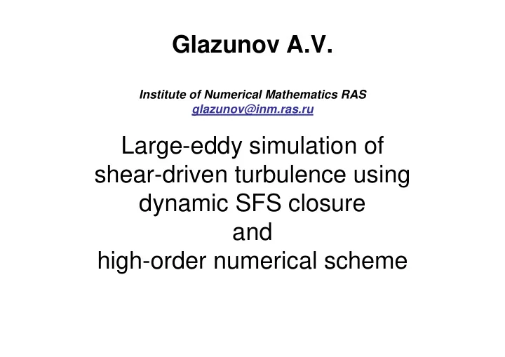
Glazunov A.V.

Institute of Numerical Mathematics RAS glazunov@inm.ras.ru

Large-eddy simulation of shear-driven turbulence using dynamic SFS closure and high-order numerical scheme

Inertial range Dissipation range Energy production range Synoptical variations Boundary-Layer flows

Now:

Modern computers are not able to do such calculations !

In the future:

Principal impossibility to specify practically applicable boundary conditions. In DNS model one needs to prescribe each leaf.

LES is the most perspective approach for practical use

DNS requirement DNS (Direct Numerical Simulation) LES (Large Eddy Simulation) RANS (Reynolds Averaged Navier-Stokes)

Three approaches for turbulence simulation

Mathematical formulation

Navier-Stokes equations.

Approximate form of the momentum and mass conservation laws in viscous incompressible fluid.

Spatial filtering

It’s usually assumed that filter commutes with operator of differentiation.

LES

Re-independent statistics of large-scale motions in turbulent flows (observation and high-Re DNS data) gives us hope of possibility:

• 1. To neglect the viscous

term.

• 2. To find closure:

) , , (

m l k ij ij

u u u Τ ≈ τ

Central problem of LES modeling. Universal approach isn’t known.

The most difficult in anisotropic wall-bounded flows (if the energy production range isn’t strongly separated from dissipation range and/or inertial range can’t be resolved by the numerical model)

It’s not always the case near the boundary and/or after discretization

The example of the particles transport by the turbulent flow among buildings Wind Particles concentration Particles are ejecting near the surface (along the dotted line). The maximal number

• f particles is about 10 000 000.

One more application (turbulent flow in domain of complex geometry ):

fraud CFD (computational fluid dynamics)

• 1. Viscous third-order finite difference approximation of nonlinear

terms in momentum balance equation.

• 2. Numerically stable but dissipative predictor-corrector time-

marching scheme.

• 3. Very simple and numerically effective K-ε closure gives results,

which are very similar to standard Smagorinsky model (far away from real turbulent stress in anisotropic turbulent flow) .

• 4. Iterative (SOR with red-black ordering) Poisson equation solver

doesn’t provide exact mass conservation. All these make the model too dissipative and incapable to reproduce properly not only the variances but even the mean values of wind velocity in complex wall-bounded turbulent flow Don’t trust such models, they don’t exist yet!

Can we return to presented simulation anytime? Let us begin with the simplest, but well-studied, anisotropic turbulent wall-bounded flow - channel flow

Stream direction Snapshot of wall-normal velocity isosurfaces ( + 1.5 U*) in rough wall bounded channel flow. LES instantaneous data (reconstructed); fragment of domain. Averaged streamwise velocity profile Two rough infinitely wide parallel plates

c

• n

s t a n t p r e s s u r e g r a d i e n t

Snapshot of wall-parallel velocity fluctuations at the centerline of rough wall bounded channel flow. LES instantaneous data (reconstructed); fragment of domain.

Some typical characteristics of channel flow

Planar averaged steamwise velocity

with the same viscosity and pressure gradient

(up to channel centerline)

Turbulent flow Laminar flow

Normalized averaged steamwise velocity (in logarithmic coordinates)

Z0 for rough- wall-bounded flow

Normalized velocity rms (up to channel centerline) Turbulent momentum flux and correlation of streamwise and wall-normal velocity Streamwise Spanwise Wallnormal

Normalized spectra of streamwise and wall-normal velocities at the different heights above surface.

invariance anisotropy Some typical characteristics of channel flow

The main requirements

1. Model should be able to reproduce mean values and variability of velocity in high-Re rough wall bounded flow. 2. Model should be applicable to the domains of complex geometry (finite-difference or finite-elements schemes) 3. Model should be suitable for parallelizing (explicit algorithms are preferable)

and restrictions

• 1. We should avoid similarity (Monin-Obukhov) arguments while the constriction of near-

the-wall model. 2. The assumption of statistical homogeneity in some spatial direction isn’t applicable (no averaging) 3. Model shouldn’t have the preferable spatial directions (3-d filtering).

The main difficulty:

Numerical errors of approximation of non-liner terms in momentum balance equation (truncation and aliasing) are of the same order or larger (for low-order schemes) than turbulent stress terms! (Ghosal, 1995, Kravchenko and Moin 1996, Park et al. 2004, Brandt 2005 …)

The dissipative up-flux schemes must be avoided due to systematic impact of numerical dissipation.

Turbulent closure

1) Eddy viscosity models (wide class of closures, includes for example: K-l, K-ε …)

Rate-of-strain tensor

Are written by analogy with molecular viscosity, but in this tensor form provide zero dissipation with solid-type rotation and not-constant KT The main advantage –provide energy cascade down to subgrid/subfilter scales The main disadvantage – don’t provide big positive correlation between real and modeled subfilter turbulent stress Very often more complicated eddy-viscosity models don’t give any improvement with respect to simplest Smagorinsky model (Neumann and Richtmyer, 1950; Smagorinsky 1963): Local balance of production and dissipation of subgrid energy Mathematically justified (Ladyzhenskaya, 1967) For the inertial range the theoretical estimation C≈0.18 exist (Lilly,1967) In standard form Smagorinsky model isn’t applicable for the modeling of wall-bounded flow (mainly due to uncertainty of coefficient C in energy production range) . Modified Smagorinsky (wall damping functions (Masson,1992) (Masson and Thomson,1992)) is slighly better

Filter width scale

Turbulent closure

2) SSM - scale-similarity model (Bardina , et al., 1983), (Sagaut, 1998),

(Layton and Lewandowski 2002): The simplest case of ADM (approximately deconvolution model):

j i j i ij

u u u u − =

* *

τ

( Stolts et.al. , 2001 ), (Gullbrand et.al.2002), (Layton, 2004) The main advantage – in the case of smooth filter provides high correlation of subfilter- scale (but not subgrid !) modeled stress with real stress. The main disadvantage – don’t produce enough dissipation.

3) MM - mixed model (Zang , et al., 1993):

Combines advantages of SSM and Smagorinsky model. But the problem of uncertainty of coefficient C still exists.

Turbulent closure

4) Dynamic approach (Germano, 1991):

Dynamic approach is based on the main assumption of the LES modelling – the invariance of turbulent closure inside some (may be quit narrow) spectral range. We suppose that one can use the same turbulent model with base model filter and with additional test filter. Invariance of the constants isn’t required in common case (scale-dependent dynamic models (Porte-Agel et al.,2000))

Germano identity:

• test filter

For the mixed model Germano identity gives:

Ratio of test filter scale to basic filter scale It’s slightly simplified formulation of dynamic model:

• 1. The numerical errors of discrete model may play the role of the additional implicit filter
• 2. The definition of the scale of smooth filters is not formulated mathematically
• 3. The spectral cut-off filter isn’t applicable in wall-normal direction
• verspecified problem with respect to C

Turbulent closure

Local in space application of Germano identity and minimizing of errors ε with least squire method gives: (+) we don’t deviate from the locality of closure. (-) ill-conditioned problem gives large amount of negative and big positive values of C. Didn’t work without additional restrictions, which are not justified physically. (-) It’s assumed that C is constant in space over entire filter width. At the case of smooth filters and/or anisotropy this assumption is questionable.

Additional minimization over: 1) Homogeneous space directions (Ghosal et al. 1995) 2) Fluid pathlines (Meneveau, et

• al. 1996).

(+) usually doesn’t give negative values of C (-) turbulent closure isn’t local ! (-) may be: gives reasonable values of C only in apriority tests and measurements, but not after including into the dynamic procedure of numerical model with very high Re.

Turbulent closure We propose:

decision variable generalized solution of

• ver-specified problem

(+) locality of closure. (+) doesn’t give large amount of negative and big positive values of C (+) reduce error ε (-) numerically expensive (consumes ~4-5 times more computational resources in comparison with ordinary dynamic model) (+) gives more smooth fields of viscosity coefficient, so permits to increase model time step

Conjugate gradients method at each time step of the model

2 4 6 8 10 12 14 16 18 20 0,40 0,42 0,44 0,46 0,48 0,50 0,52 0,54 0,56 0,58

iteration v

τ ε

Conjugate gradients method Local least-squire method

2 2

( ) 1 2

ij ij ij s ij ij

L H M C M M − = − ∆

2 2

(2 ) ( )

T T s

A A C A L H ∆ = −

The areas with restricted values are not colored

s xy

C

2 2

(2 ) ( )

T T s

A A C A L H ∆ = −

2 2 2 max 2

( ) 1 , 2

ij ij ij s s s ij ij

L H M C C C M M − = − ≤ ≤ ∆

2 2

( ) 1 2

ij ij ij xy s ij ij xy

L H M C M M − = − ∆

2 2

( ) 1 2

ij ij ij xy s ij ij xy

L H M C M M − = − ∆ Vertical profiles of averaged value of C, computed by the different methods

A posteriori minimizing over spatially homogeneous directions gives results proportional to conjugate gradients method Minimizing over spatially homogeneous directions included into dynamic procedure strongly underestimates dissipation near the wall.

Boundary conditions

2d-periodic in spanwise and streamwise directions.

Local similarity at the bottom and top walls: This additional constraints are not needed for the closed form of the model equations, but are used inside the dynamic procedure (grid is staggered -S13 and S23 are not defined at z=1/2Δz ) Provides good correspondence with logarithmic profiles in vicinity of surface

Due to local logarithmicity Due to white-noise spectrum and constant rms of wall normal velocity in vicinity of surface

(-) local logarithmicity of wall-parallel velocity is not justified physically (-) doesn’t provide integral equivalence with Monin-Obukhov theory (-) boundary conditions are not involved into dynamic procedure (+?) by our experience it’s still better choice of wall-model, which doesn’t suppress the variability at the closest to surface levels.

λ

U

2-order central difference scheme 4-order central difference scheme

Modified advection velocity in 2-d and 4-th order central difference schemes Small-scale fluctuations of velocity remain behind the average flow and can be destroyed on the dissipative terms of subgrid (subfilter) closure. This mechanism works as an additional implicit filter in streamwise direction. This effect is more crucial for low-order schemes.

Fully conservative 4-order central difference scheme (Morinishi et.al.,1998) (Vasilyev, 2000)

Staggered grid Skew-symmetric form Direct Poisson equation solver (would to be modified for complex geometry) Easy to be parallelized (only 2 extra grid points are required)

Are equivalent for nonlinear terms, but skew- symmetric is preferable for using inside SSM

All approximations of viscous terms are 4-th order too (impotent) Scale similarity part of closure is calculated using the advection scheme

i i i

u P H t x δ δ ∂ = − + ∂

* 1

3 1 1. 2 2

n n n i i i i

u u t H H

−

  − = ∆ −    

* 2 2

1 2.

j i j

u P x t x δ δ δ δ   =     ∆  

1 *

3.

n i i i

P u u t x δ δ

+ =

− ∆

Direct and inverse 2-d FFT with the appropriate modified wave-numbers in “x-y” plane Septa-diagonal solver of Nx*Ny liner equations 4-times transposition of data (2d/3d → 1d decomposition and backwards) for the parallel computing.

Temporal approximation

Adams-Beshfort scheme, ”fractional-step” method 2-d order of accuracy (not conserved) liner growth of energy can be reduced with the small steps (in our calculation Δt ~ 0.1-0.2 CLF)

Parallel implementation

MPI-based realization –oriented to the supercomputers with distributed memory. (easy transferable between different computers). Each process contains only the information about the single sub-domain + several boundary extra-points (no problems with memory restrictions). Non-blocking exchanges. Possibility to exchange only the needed plate, edge or corner. 3 or 2 –decomposition of computational domain. (for the channel flow 2-d decomposition is preferable)

Tested and implemented at 32-processors Intel Itanium2 cluster of INM RAS and computational resources of Joint SuperComputer Center For the large domains speedup ~ 12 at 16 nodes.

0,0 0,1 0,2 0,3 0,4 0,5 0,6 0,7 0,8 0,9 1,0 0,0 0,2 0,4 0,6 0,8 1,0

G(k)

∆k/π

Filters

3-points approximations of top-hat filter

basic filter (

_)

test filter (^) (widest among 3-point explicit filters) production of test and basic filters (^)

More often used choice - 3-point approximation of Gauss filters with more smooth transfer functions isn’t wide enough and leads to big numerical errors in our experiments Wide top-hat filter (Katapodes et al. 2005) inverts short-wave harmonics and isn’t applicable too. Any nonsymmetrical filter in vicinity of surface produces faze shifts.

α2 = 4 (for inner region) – this choice isn’t justified mathematically (more justified - α2 = 5) but we don’t know how the implicit filtering works! α2 = 4 2/3 (for the nearest to wall level) – (appropriate 2d filters are used).

(-) Filters are smooth and suppress all harmonics (-) Basic filter doesn’t sufficiently suppress short-wave side of spectra with largest numerical errors (-) α –remains to be the model parameter (+) Simplicity and numerical efficiency

SE

Viscous dissipation

kDNS k kLES

grid

∆

Filter

USFS

2

1 2 3

ij ij kk ij

С S S τ δ τ − =− ∆ | |

ij i j i j

u u u u τ = −

SGS NE

4

( )

i j grid j

u u

• x

∂ + ∆ ∂

RSFS forcing How should it work ?

Lx/h=18,28 ~ 5,8 π, Ly/h=4,57 ~ 1,45 π, (Δx: Δy: Δz) = (1 : 1 : 0.875), 512x128x64 Lx/h=27,42 ~ 8,7 π, Ly/h=9,14 ~ 2,9 π, (Δx: Δy: Δz) = (1 : 1 : 0.875) 768x256x64 Lx/h=18,28 ~ 5,8 π, Ly/h=9,14 ~ 2,9 π, (Δx: Δy: Δz) = (2 : 2 : 0.875), 256x128x64

Non-dimensional wall normal gradient of averaged streamwise velocity

Color lines – LES with different grid resolutions and domain sizes. Black lines – DNS with different Re_τ (up to Re_τ = 2003) Dots with error bars - High Reynolds Princeton Superpipe data (McKeon et al., 2004)

DNS LES DATA z/h

“Log-wake law” (W –universal Re-independent function)

0,2 0,4 0,6 0,8 1,0 1,2 1,4 2 4 6 8 10 12

(Ucl-U)/U* z/h

0,1 1 2 4 6 8 10 12

(Ucl-U)/U* z/h

Defect of average streamwise velocity (U_cl-U)/U* (U_cl - velocity at the channel centerline)

Color lines – LES with different grid resolutions and domain sizes. Dots - High Reynolds Princeton Superpipe data (Re = 3.5724E+07 )

http://gasdyn.princeton.edu/data/e248/mckeon_data.html

Lx/h=18,28 ~ 5,8 π, Ly/h=4,57 ~ 1,45 π, (Δx: Δy: Δz) = (1 : 1 : 0.875), 512x128x64 Lx/h=27,42 ~ 8,7 π, Ly/h=9,14 ~ 2,9 π, (Δx: Δy: Δz) = (1 : 1 : 0.875) 768x256x64 Lx/h=18,28 ~ 5,8 π, Ly/h=9,14 ~ 2,9 π, (Δx: Δy: Δz) = (2 : 2 : 0.875), 256x128x64

(LES resolved) Normalized velocity rms

Lx/h=18,28 ~ 5,8 π Ly/h=4,57 ~ 1,45 π (Δx: Δy: Δz) = (1 : 1 : 0.875) 512x128x64

Variances of all three components of resolved velocity are strongly underestimated!

Vertical velocity variance falls down to surface. Spanwise variance doesn’t grow near the wall.

Subgrid scales can’t contain energy enough to compensate differences! z/h

High-Re DNS data

LES

( mixed dynamic closure, finite difference, 4-th order in space, 2-d order explicit in time) 512 x 128 x 64 = 4 194 304 grid points (Δx: Δy: Δz) = (1 : 1 : 0.875) Lx/h=18,28 ~ 5,8 π Ly/h=4,57 ~ 1,45 π (t u*)/h ~ 16 ~ 150 hours (2400 processor-hours) in 16 processors (cluster INTEL ITANIUM, INM RAS)

DNS (LES reconstructed) Normalized velocity rms (u*≈F-1ū, F=(

_) – base model filter)

z/h

Correlation of streamwise and wall- normal velocities up to channel centerline LES reconstructed LES resolved Planar and time-averaged components of momentum flux in constant-pressure gradient driven channel flow (LES data) Total flux Resolved + SMM+SSM Resolved flux Total subgrid/subfilter flux Subfilter flux, produced by scale-similarity part of closure Viscous part of flux, produced by Smagorinsky part of the closure

h z

2 *

/u τ

h z

2 / 1 2 2 / 1 2

' ' ' ' w u w u

Reconstructed correlation is slightly closer to expected value 0.4

Instantaneous planar averaged components of momentum flux.

Resolved flux computed using the reconstructed field of velocity Total subgrid/subfilter flux Subfilter flux, prodused by SSM Viscous part of flux, produced by Smagorinsky part of the closure Total flux Resolved + SMM+SSM Resolved flux

The momentum flux computed by the reconstructed field of velocity and total flux practically coincide! The reconstructed variability isn’t random fluctuation, but well correlated pulsations which provide reasonable momentum exchange

10

• 2

10 10

• 2

10

• 1

10 10

1

10

2

lev=1 z/h=0,0156 z/h=0,047

k

• 5/3

E(u1,u1)u*

• 2/z

λx=5∆x

k

• 1

kxz

z/h=0,14 z/h=0,48 lev=16 z/h=0,36 z/h=0,27 z/h=0,2 z/h=0,11 z/h=0,078

Normalized energy spectra of streamwise velocity fluctuation versus nondimensional streamwise wavenumber. LES produced filtered velocity.

Lx/h=18,28 ~ 5,8 π Lz/h=4,57 ~ 1,45 π (Δx: Δy: Δz) = (1 : 1 : 0.875) 512x128x64

No invariance ! No power law !

Are the results Re_model dependent ?

10

• 2

10 10

• 2

10

• 1

10 10

1

10

2

z/h=0,14 z/h=0,48 z/h=0,36 z/h=0,27 z/h=0,2 z/h=0,11 z/h=0,078

z/h=0,047 lev=2 z/h=0,0156 lev=1

E(u*

1,u* 1)u*

• 2/z

k

• 5/3

k

• 1

kxz

λx=5∆x

Normalized energy spectra of streamwise velocity fluctuation versus nondimensional streamwise wavenumber. Reconstructed velocity. (u*≈F-1ū, F=(

_) – base model filter) Lx/h=18,28 ~ 5,8 π Lz/h=4,57 ~ 1,45 π (Δx: Δy: Δz) = (1 : 1 : 0.875) 512x128x64

(+) Invariance

(-) except of second computational level.

• 1. Drawback of model

(+) Power dependence in wide region

(-) The slope

• f spectrum is

slightly less than (-5/3) (best fit ~ (-5/3+1/8))

• 1. Drawback of model?
• 2. Real physics in narrow

spectral interval ?

• 3. Influence of opposite

wall? (-) Spectral maxima is not reached

• 1. Insufficient length of

computational domain?

• 2. Drawback of model

(unphysical boundary condition)? (+) Sharp (-) cutoff of spectrum at k=2π/(5Δ)

• 1. Implicit filtration due to

finite difference errors?

• 2. Drawback of model?

Lx/h=27,42 ~ 8,7 π Lz/h=9,14 ~ 2,9 π (Δx: Δy: Δz) = (1 : 1 : 0.875) 768x256x64

Normalized energy spectra of streamwise velocity fluctuation versus nondimensional streamwise wavenumber. LES data. Reconstructed velocity. Velocity spectra obtained in a turbulent pipe (Re=2.0E5) (Perry et al.,1986) Enlarged fragment of experimental data, corresponding to LES spectral range. Good correspondence with the observed spectra We simulate quit narrow region of real variability The domain size is still insufficient for representation

• f low-frequency variability

10

• 1

10 10

1

10

• 2

10

• 1

10 10

1

lev=16 z/h=0,48 lev=1 z/h=0,0156

grid cutoff

E(u*

1,u* 1)u*

• 2/z

k

• 5/3

k

• 1

kyz

Normalized energy spectrum of streamwise velocity fluctuation versus nondimensional spanwise wavenumber. LES produced filtered velocity.

No invariance ! No power law !

10

• 1

10 10

1

10

• 2

10

• 1

10 10

1

z/h=0,047 lev=2 lev=16 z/h=0,48 lev=1 z/h=0,0156 grid cutoff

E(u*

1,u* 1)u*

• 2/z

k

• 5/3

k

• 1

kyz

Normalized energy spectra of streamwise velocity fluctuation versus nondimensional spanwise wavenumber. Reconstructed velocity. (u*≈F-1ū, Fˇ (

_) – base model filter) Lx/h=18,28 ~ 5,8 π Lz/h=4,57 ~ 1,45 π (Δx: Δy: Δz) = (1 : 1 : 0.875) 512x128x64

(+) Invariance

(-) except of second (and nearest to second) computational levels short-wave modes.

• 1. Drawback of model

(+) Power dependence in wide region up to grid cutoff (+) Inertial range E~k^(-5/3) is reproduced with high accuracy

(-) Accumulation of energy in long-wave harmonics

• 1. Insufficient length of

computational domain?

• 2. Drawback of model

(unphysical boundary condition)?

10 10

1

10

• 3

10

• 2

10

• 1

10

E(u

1,u 1)

domain size 2 cutoff domain size 1 cutoff grid 2 cutoff E(u

*

1,u

*

1)

~k

• 5/3

E(u1,u1)u*

• 2/h

k

yh

z=h/2 grid 1 cutoff

Spanwise normalized one-dimensional energy spectra of streamwise velocity fluctuation at z=h/2 with different grid resolutions and domain sizes. Original filtered (LES reproduced) - thin lines. Reconstructed - bold lines and dots. (+) Invariance of reconstructed statistics with respect to grid resolution

(The basic assumption

• f LES approach)

(-) The domain sizes are insufficient for invariance of low-frequency spectrum intervals. In DNS modeling the same domain-side aspect ratios are successfully used. 1. Drawback of the model? 2. Dependence of position of spectrum maxima on external dimensional parameter z0 ? If (2) – we should use even larger computational domains to reach really true statistics and compare the LES models and closures but not the consequences of “infrared catastrophe”

10 10

• 2

10

• 1

10 10

1

~k

• 5/3

~k

• 1

S33u*

• 2/z

k1z

Normalized energy spectra of wall-normal velocity versus nondimensional streamwise wavenumber (reconstructed velocity).

Best fit – Ew =0.4u*

2k-1

LES (from the fist computational level up to channel centerline)

Two-dimensional normalized energy spectrum of streamwise velocity fluctuation

Lx/h=18,28 ~ 5,8 π Lz/h=9,14 ~ 2,9 π (Δx: Δy: Δz) = (2 : 2 : 0.875) 256x128x64 z=0.5h Lx/h=18,28 ~ 5,8 π Lz/h=4,57 ~ 1,45 π (Δx: Δy: Δz) = (1 : 1 : 0.875) 512x128x64

Two-dimensional normalized energy spectrum of streamwise velocity fluctuation

Lx/h=27,42 ~ 8,7 π Lz/h=9,14 ~ 2,9 π (Δx: Δy: Δz) = (1 : 1 : 0.875) 768x256x64 z=0.5h

Lx/h=27,42 ~ 8,7 π Ly/h=9,14 ~ 2,9 π (Δx: Δy: Δz) = (1 : 1 : 0.875) 768x256x64

Two-dimensional normalized energy spectrum of spanwise velocity fluctuation Two-dimensional normalized energy spectrum of wall-normal velocity fluctuation

At the beginning of this report I crossed out the results with the flow among buildings On the next slide I’ll do similar thing with the results presented just now

“Sliding” model

System of coordinates is moving with the constant velocity in the direction of the flow, the boundary conditions are modified to preserve the original fluxes

10

• 1

10

1

10

• 3

10

• 2

10

• 1

10 10

1

10

2

<U>xy > 0 <U>xy < 0

E(u

*

1,u

*

1)u*

• 2/z

grid cutoff <U>xy ~ 0 z/h = 0,075

~k

• 5/3

~k

• 1

k1z

We have lost the invariance! The single spectrum which shows expected power laws (up to grid cutoff) is the spectrum at the height with zero mean velocity The implicit filter due to numerical errors still plays a significant role

The model is not invariant under Galilean transformation

Developed LES model is able to reproduce the dynamics of rough-wall bounded channel flow with good accuracy. (+) Only the reconstructed velocity shows the required statistics. So: 1) SSM part of the closure provides adequate subfilter part of the turbulent stress 2) Dissipative Smagorinsky-type part of the closure combined with the original dynamic procedure provides well-balanced dissipation in anisotropic flow. 3) High-order conservative numerical scheme is able to reproduce filtered dynamic of turbulent flow up to wave-lengths approximately equal to 5 grid steps. 4) Implicit filter (numerical errors + viscous part of the closure) works as a sharp cutoff filter in steamwise direction. 5) All developed numerical algorithms are applicable for the flows in domains of complex geometry (except for Poisson equation solver, but it’s a technical and easy solvable problem)

But: The model is not invariant under Galilean transformation -- the implicit numerical filtration still plays significant role in model dynamics. So:

We should be very carefull with implementation of this model in the complex domains

CONCLUSIONS

Future plans and possible ways of problems solution

1) Explicit filtering with sufficiently wide commutative filters in the inner part of the flow. 2) Symmetric filters with variable width (reduced near the wall) together with explicit modeling of commutative errors. 3) Involving of the boundary conditions into the dynamic procedure. 4) Dynamic determination of the single model parameter – the ratio of filters widths.