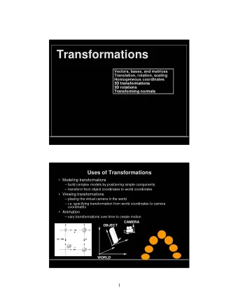
geometric transforms 1 linear algebra review 2 matrices matrix - PowerPoint PPT Presentation

geometric transforms 1

linear algebra review 2

matrices matrix and vector notation use column for vectors m 11 m 12 M = [ ] = [ m ij ] m 21 m 22 T v 1 v = [ ] = v 1 v 2 [ ] v 2 3

matrix operations addition T = M + N t ij ] = [ m ij + n ij [ ] scalar multiplication T = aM t ij ] = [ am ij [ ] 4

matrix operations matrix-matrix multiplication row-column multiplication not commutative associative m ik n kj T = MN = [ t ij ] = [ ∑ ] k ⎡ ⎤ ⎡ ⎤ ⎡ ⎤ t 11 t 12 m 11 m 12 n 11 n 12 ⎢ ⎥ ⎢ ⎥ ⎢ ⎥ = ⎢ ⎥ ⎢ ⎥ ⎢ ⎥ ⎣ ⎦ ⎣ ⎦ ⎣ ⎦ m 21 m 22 n 21 n 22 t 21 t 22 5

matrix operations matrix-vector multiplication row-column multiplication u = M v ⎡ ⎤ ⎡ ⎤ ⎡ ⎤ u 1 m 11 m 12 v 1 ⎢ ⎥ ⎢ ⎥ ⎢ ⎥ = ⎢ ⎥ ⎢ ⎥ ⎢ ⎥ ⎣ ⎦ ⎣ ⎦ ⎣ ⎦ u 2 m 21 m 22 v 2 6

matrix operations transpose: flip along diagonal T = M T t ij ] = [ t ji [ ] inverse (not computed explicitly in this course) T = M −1 M −1 M −1 MT = M = M = I 7

special matrices identity: invariant for multiplication 1 i = j I = [ i ij ] = { 0 i ¡ j 1 0 I = [ ] 0 1 : M : M = MI = IM 8

special matrices zero: invariant for addition O = [ i ij ] = 0 0 0 I = [ ] 0 0 : M : M = M + O = O + M 9

matrix operation properties linearity of multiplication and addition a ( A + B ) = aA + aB M ( aA + bB ) = aMA + bMB associativity of multiplication A ( BC ) = ( AB ) C 10

matrix operation properties transpose and inverse of multiplication ) T B T A T ( AB = ) −1 B −1 A −1 ( AB = 11

2d transformation 12

geometric transformations functions that maps points to points p ′ p Ü = X ( p ) different transformations have restrictions on the form of X 13

translation T t ( p ) = p + t T −1 ( p ) = T − t ( p ) = p − t t 14

linear transformations fundamental property: X ( a p + b q ) = aX ( p ) + bX ( q ) can be represented in matrix form: X ( p ) = M p properties: maps origin to origin maps lines to lines parellel lines remain parallel length ratios are preserved closed under composition 15

uniform scale p x sp x s 0 S s p = [ ] = [ p y sp y ][ ] 0 s S −1 = S 1/ s s 16

non-uniform scale s x 0 p x s x p x S s p = [ ] = [ p y s y p y ][ ] 0 s y S −1 = S 1/ s s 17

rotation p x cos ? − p y sin ? p x cos ? − sin ? R ? p = [ ] = [ p y ][ sin ? cos ? p x sin ? + p y cos ? ] R −1 = R − ? ? 18

shear p x + s x p y 1 s x p x S h s p = [ ] = [ p y ][ s y 1 s y p x + p y ] 19

reflection p x − p x −1 0 R p = [ l x ] = [ ] R p = ) l y p y p y ][ 0 1 p x − p x −1 0 R p = [ l o ] = [ ][ p y − p y ] 0 −1 20

affine transforms combine translation with linear transformation rigid body transformation are a subset of this X M , t ( p ) = M p + t properties does not map origin to origin maps lines to lines parallel lines remain parallel length ratios are preserved closed under composition 21

transforming points and vectors points and vectors are different entities vectors: encode direction and length (difference of points) points: encode position (origin plus a vector) points: transform as reported above X ( p ) = M p + t vectors: transform like points, but no translation is applied X ( v ) = M v directions (normalized vectors): normalize after transform ^ ^ ^ X ( ) = M /| M | d d d 22

transforming points and vectors proof that vectors transform as such v = p − q X ( p ) = M p + t X ( v ) = X ( p ) − X ( q ) = = ( M p + t ) − ( M q + t ) = = M ( p − q ) = = M v 23

homogeneous coordinates represent points/vectors with an additional coordinate w set it to 1 for points (or multiply all per arbitrary ) w ⎡ ⎤ p x ⎡ ⎤ wp x ⎢ ⎥ ⎢ ⎥ p y p = ¢ wp y ⎢ ⎥ ⎢ ⎥ ⎣ ⎦ ⎣ ⎦ w 1 set it to 0 for vectors ⎡ ⎤ v x ⎢ ⎥ v y v = ⎢ ⎥ ⎣ ⎦ 0 24

homogeneous coordinates translation: represent as 3x3 matrix ⎡ ⎤ ⎡ ⎤ ⎡ ⎤ 1 0 t x p x p x + t x ⎢ ⎥ ⎢ ⎥ ⎢ ⎥ p y p y + t y 0 1 t y T t p = = ⎢ ⎥ ⎢ ⎥ ⎢ ⎥ ⎣ ⎦ ⎣ ⎦ ⎣ ⎦ 0 0 1 1 1 shorthand notation for points and vectors p p + t I t T t p = [ ] = [ ][ ] 0 1 1 1 I t v v T t v = [ ][ ] = [ ] 25 0 1 0 0

homogeneous coordinates linear transform: 3x3 matrix by adding one row,column ⎡ ⎤ ⎡ ⎤ m 11 p x + m 12 p y ⎡ ⎤ p x m 11 m 12 0 ⎢ ⎥ ⎢ ⎥ ⎢ ⎥ p y M p = = m 21 p x + m 22 p y m 21 m 22 0 ⎢ ⎥ ⎢ ⎥ ⎢ ⎥ ⎣ ⎦ 0 0 1 ⎣ ⎦ ⎣ ⎦ 1 1 shorthand notation for points and vectors p M p M 0 M p = [ ] = [ ][ ] 0 1 1 1 M 0 v M v M v = [ ][ ] = [ 26 ] 0 1 0 0

affine transformations combine linear and translation in one matrix p M t X p = [ ] = M p + t ][ 0 1 1 M t v X v = [ ][ ] = M v 0 1 0 27

combining transforms apply one transformation after the another express by function composition p ′ = X 2 X 1 ( ( p )) = ( X 2 Q X 1 ( p )) for affine transformations, compute by matrix multiplication ( X 2 Q X 1 ( p )) = X 2 X 1 ( ( p )) = M 2 M 1 ( ) p = ( M 2 M 1 ) p 28

combining transforms translation I t 2 I t 1 I t 1 + t 2 ] = [ [ ][ ] 0 1 0 1 0 1 linear transformations M 2 0 M 1 0 M 2 M 1 0 ] = [ [ ][ ] 0 1 0 1 0 1 29

combining transforms affine transformations M 2 t 2 M 1 t 1 M 2 M 1 M 2 t 1 + t 2 ] = [ [ ][ ] 0 1 0 1 0 1 30

composition is not commutative original rotation translation original transation rotation 31

complex transformations represent as combination of simpler ones intuitive geometric interpretation rotation around arbitrary axis at of angle a ? translate axis center to origin rotate (about origin) translate back R a , ? = T a R ? T − a 32

complex transformations 33

complex transformations 34

transforms and coordinate systems change of coordinate system can be written as affine matrix for , we have f ′ f ′ x f ′ x f ′ x f ′ p ′ p ′ p ′ Ü f p = + + + O x y z that in matrix form becomes f ′ f ′ f ′ f ′ p ′ p ′ M t x y z o p = [ ] = [ ][ ] [ ] 0 1 1 1 0 0 0 1 35

transforms and coordinate systems for , we invert the previous equation f Ü f ′ M −1 M −1 p t p ′ = [ ][ ] 0 1 1 since is orthonormal, M −1 M T M = x ′ T x ′ ⎡ ⎤ ⎡ ⎤ ˝ t p x ⎢ ⎥ ⎢ ⎥ y ′ T y ′ p y ˝ t ⎢ ⎥ ⎢ ⎥ p ′ = ⎥ ⎢ ⎥ ⎢ z ′ T z ′ p z ˝ t ⎢ ⎥ ⎢ ⎥ ⎣ ⎦ ⎣ ⎦ 1 0 1 36

3d transformations 37

3d transformations adopt homogeneous formulation in 3d point have 4 coordinates use 4x4 matrices for transformations most concepts generalize very easily rotation much more complex 38

translation ⎡ ⎤ 1 0 0 t x ⎢ ⎥ 0 1 0 t y ⎢ ⎥ T t = ⎢ ⎥ 0 0 1 t z ⎢ ⎥ ⎣ ⎦ 0 0 0 1 39

scale ⎡ ⎤ s x 0 0 0 ⎢ ⎥ 0 s y 0 0 ⎢ ⎥ S s = ⎢ ⎥ 0 0 s z 0 ⎢ ⎥ ⎣ ⎦ 0 0 0 1 40

rotation around z ⎡ ⎤ cos ? −sin ? 0 0 ⎢ ⎥ sin ? cos ? 0 0 R z ⎢ ⎥ = ? 0 0 1 0 ⎢ ⎥ ⎣ ⎦ 0 0 0 1 41

rotation around y ⎡ ⎤ cos ? 0 sin ? 0 ⎢ ⎥ 0 1 0 0 R y ⎢ ⎥ = ? −sin ? 0 cos ? 0 ⎢ ⎥ ⎣ ⎦ 0 0 0 1 42

rotation around x ⎡ ⎤ 1 0 0 0 ⎢ ⎥ 0 cos ? −sin ? 0 R x ⎢ ⎥ = ? 0 sin ? cos ? 0 ⎢ ⎥ ⎣ ⎦ 0 0 0 1 43

rotation around arbitrary axis in 2D, rotation are around a point: R a , ? = T a R ? T − a change coordinate frame (translation) rotation around the origin change coordinate frame back simple geometric construction in 3D, rotation are around an axis: F − 1 a R ? F a R a , ? = change coordinate frame (align with axis ) z a rotation around z change coordinate frame back complex geometric construction 44

representing rotations Euler angles: 3 rotations around major axis remember to choose order simple but has quirks when combining rotations will use this for simplicity axis and angle combinations of rotations can be represented this way with more formalism become elegant and consistent quaternions 45

transforming normals points and vectors works tangents, i.e. differences of points, work too normals works differently defined as orthogonal to the transformed surface i.e. orthogonal to all tangents 46

transforming normals by definition: t T t ˝ n = n = 0 after tranform: ) T ( M t ( X n ) = 0 for all we have: t T M T t X n = 0 which gives: t T M T M T ) −1 ( n = 0 normals are transformed by the inverse transpose 47

transformation hierarchies 48

transformation hierarchies often need to transform an object wrt another e.g. the computer on the table when the table moves, the computer moves naturally build a hierarchy of transformation to transform the table, apply its transform to transform the computer, apply the table and the computer transform 49