GeoCom putational I ntelligence and GeoCom putational I ntelligence - PowerPoint PPT Presentation

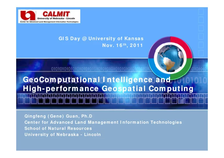
GI S Day @ University of Kansas Nov. 1 6 th , 2 0 1 1 GeoCom putational I ntelligence and GeoCom putational I ntelligence and High-perform ance Geospatial Com puting High-perform ance Geospatial Com puting Qingfeng ( Gene) Guan, Ph.D Center for Advanced Land Managem ent I nform ation Technologies School of Natural Resources University of Nebraska - Lincoln

Contents 1. Computational Science and GeoComputation 2. GeoComputational Intelligence - ANN-based Urban-CA model 3. High-performance Geospatial Computing - Parallel Geostatistical Areal Interpolation - pRPL and pSLEUTH 4. Conclusion

I ntroduction – Com putational Science  Definition  “ the field of study concerned with constructing mathematical models and numerical solution techniques and using computers to analyze and solve scientific, social scientific and engineering problems.” (wikipedia)  Dom ains include:  Numerical simulations  Model fitting and data analysis  Massive com putational intensity http://www.it.uu.se/edu/masters/CompSc/

I ntroduction - GeoCom putation  Definition  Couclelis (1998) identified the “core GeoComputation” as the innovative (or derived from other disciplines) computer-based geospatial modeling and analysis Contrasted against the traditional computer-supported spatial data analysis and geospatial modeling  Openshaw (2000) also emphasized Computational Science as the origin of GeoComputation (the Computation part) and the essential concerns about geographical and earth systems (the Geo part)  The capital G and C

I ntroduction – GeoCom putation ( cont.)  Methodology  A wide array of computer-based models and techniques, many of them derived from the field of Artificial Intelligence (AI) and the more recently defined area of Computational Intelligence (CI) (Couclelis, 1998) • Expert Systems, Cellular Automata, Neural Networks, Fuzzy Sets, Genetic Algorithms, Fractal Modelling, Visualization and Multimedia, Exploratory Data Analysis and Data Mining, etc.  High-perform ance geospatial com puting

ANN-Urban-CA: an urban grow th m odel  Overview  Combination of a Cellular Automata (CA) model, an Artificial Neural Network (ANN), and a macro-scale socio-economic model  Integration of Geography, Natural Resource Science, Social Science, and Economics in a GeoComputation framework

Geospatial Cellular Autom ata  Bottom -Up structure  Simple local rules to simulate complex global spatio-temporal dynamics  W idely used in geospatial m odeling  Land-use/Land-cover Change  Wildfire Propagation  Flood Spreading  Freeway Traffic Flow Prediction of urban development to the year 2050 over southeastern  More and More Coming up… Pennsylvania and part of Delaware using the SLEUTH model http://www.essc.psu.edu/~dajr/chester/ animation/movie_small.htm

I ssues of Geospatial CA  Hard to set proper transition rules and param eters  How to produce realistic simulations?  Brute-force calibration • Generate results using all possible parameter values • Find the “best-match” combination • Highly computationally intensive  Lack of global control  Bottom-up structure  Evolve without constraints

ANN-Urban-CA: Structure  An Artificial-Neural-Netw ork-Based, constrained, Cellular Autom ata m odel for urban grow th sim ulation

ANN-Urban-CA: ANN  Artificial Neural Netw ork  ANN is suited for dealing with complex nonlinear relationships, e.g., the impacts of driving factors to urban growth  ANN can learn from available data, and deal with redundancy, inaccuracy, and noise  Knowledge and experience can be easily learned and stored for further simulation

ANN-Urban-CA: Macro Constrain  Macro-scale Socio-econom ic m odel  The Tietenberg model is used to generate the proper demand for urban space in each period (e. g. year) in the future.  A Resource Economic model, which usually is used to solve the problem of   a bq / P c “ how to consume resources in the    t ta 0 future according to the principle of   t 1 r sustainable development ” ( 1 )  Lands are treated as non-  regenerative resources, and the  t n ( 1 , 2 , , ) urbanization process is treated as land source consumption  Population increase as the driving n    force of land consumption Q q 0 t  t 1

ANN-Urban-CA: Training  Purpose  ANN adjusts the weight values  Determine the best-fit transition rules and parameters of the CA  Method  Back-Propagation (BP) training algorithm  Input: Driving factors  Output: Urbanization probability  Target: Historical urban data

ANN-Urban-CA: Results Real Beijing urban, 2000  History Sim ulation  Trained using samples of Beijing urban maps of 1980, 1995, and 2000  Simulate urban growth in Beijing 1995 - 2000  A A    real sim Lee Sallee 0.8318  A A real sim n  c ij   k correlatio n 0.9018 n n      2 2 ( z z ) ( z z ) i i j j k k Simulated Beijing urban, 2000

ANN-Urban-CA: Results  Future Forecast 1400 1200 Simulated Urban  Increased populations of 1000 Population Beijing 2001- 2015 800 Real Urban 600 Population  By using the Tietenberg 400 Model, 6 scenarios of 200 urbanization were derived 0 1978 1981 1984 1987 1990 1993 1996 1999 2002 2005 2008 2011 2014 Increased Pop Total Scenario 1 Total Scenario 2 Total Scenario 3 （ Years （ 10,000 ） （ hm 2 ） （ hm 2 ） hm 2 ） r=0 r=0.01 r=0 r=0.01 r=0 r=0.01 2001 ～ 2005 123.956 7522.9 8201.1 15186.8 15781.6 17741.5 18308.5 2006 ～ 2010 141.766 8687.9 8758.7 17538.6 17600.8 20488.8 20548.1 2011 ～ 2015 162.134 10033.2 9284.2 20254.6 19597.6 23661.7 23035.4

ANN-Urban-CA: Results Urban Growth in Beijing 2000 – 2015 (Scenarios 1)

ANN-Urban-CA: Results Urban Growth in Beijing 2000 – 2015 (Scenario 4)

Sub-Conclusion on ANN-Urban-CA  ANN’s capability of dealing w ith nonlinear com plex system s  Calibrated without heavy computing overhead and subjective human interference  Optim al quantity allocation + optim al spatial allocation  Providing an ideal pattern of sustainable urban development, useful in urban planning  Highly flexible structure and m odeling approach  Easily generalized to model other kinds of spatio-temporal dynamics for various purposes, e.g., spread of invasive species and vegetative epidemics, movement of toxic pollutants in water systems, and land-cover change caused by climate change  Open to any possible/available datasets, e.g., numerous remotely sensed data and other natural resource and environmental data

High-perform ance Geospatial Com puting  W hy high-perform ance com puting?  GeoComputation implies HPC  Increasing demand for computational power in geospatial research and applications – Sophisticated and complicated analytical algorithms and simulation models – High-resolution and large-volume datasets – Rapid processing and real-time response

High-perform ance Com puting  Definition  Usually refers to parallel computing • The use of multiple computing units (e.g., computers, processors/CPU cores, or processes) working together on a common task in a concurrent manner in order to achieve higher performance • In contrast to sequential computing that usually has only one computing unit  Performance is usually measured with computing time  Em erging Cyberinfrastructure A massive parallel computing system  Grid Computing (http://ctbp.ucsd.edu/pc/html/i  Cloud Computing ntro4.html )

Areal I nterpolation – I ntroduction Population of counties  Definition 6 x 10 4.6  Predicts the unknown (target) attribute values 4.5 4.4 at the required partition (target zones or 4.3 4.2 supports) from a set of known (source) 4.1 4 attribute data available on a different partition 3.9 3.8 (source zones or supports) 3.7 3.6  Tw o m ain approaches 0 2 4 6 5 x 10 Population of watersheds = ?  Cartographical methods 6 x 10 4.6 • Use cartographical properties of supports, e.g., 4.5 area, as the basis 4.4 4.3 • Simple and widely used 4.2 4.1  Geostatistical methods 4 3.9 3.8 • Use variants of Kriging 3.7 3.6 • Accounts for spatial autocorrelation 0 2 4 6 5 x 10 • Measure the reliability of prediction An areal interpolation problem • Mass-preserving target prediction

Geostatistical Areal I nterpolation  Steps  Discretization of source and target supports with a regular raster (point values not known, just location)  Computation of support-to-support covariances as integrals from a given point covariance model • Between all source supports • Between all source and target supports  Use of Kriging system with computed covariances to derive weights for interpolation  Interpolated values computed as linear combinations of the Kriging weights and the source data