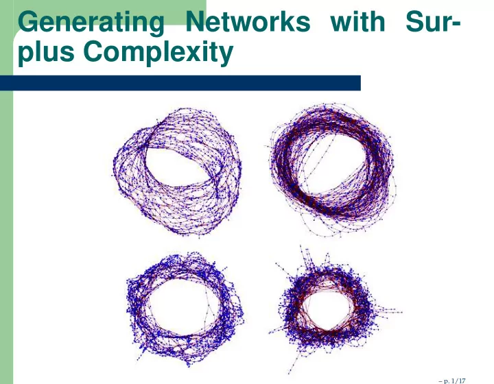
Generating Networks with Sur- plus Complexity p. 1/17 Complexity, - PowerPoint PPT Presentation

Generating Networks with Sur- plus Complexity – p. 1/17

Complexity, or amount of infor- mation Note: Information = data + meaning Meaning B Meaning A Semantic Space “B is more complex than A ������������������� ������������������� ������������������� ������������������� ������������������� ������������������� B ��� ��� ������������������� ������������������� Syntactic Space ��� ��� ������������������� ������������������� ���� ���� ��� ��� A ������������������� ������������������� ���� ���� ������������������� ������������������� N letters in alphabet ���� ���� ������������������� ������������������� ���� ���� ������������������� ������������������� ���� ���� ������������������� ������������������� descriptions of length ℓ ������������������� ������������������� – p. 2/17

Complexity as Information We need two things to determine the complexity of something: � An encoding over a finite alphabet (eg a bitstring) � A classifier function (aka observer) of the strings that can determine whether two encodings refer to the same object – p. 3/17

Kolmogorov complexity of a bit- string � Classifier is a Turing machine � Encodings are programs of the Turing machine that output the thing (a bitstring) � In the limit as n → ∞ , complexity is dominated by the length of the shortest program (compiler theorem). � Random strings are maximally complex – p. 4/17

Effective complexity of English literature � Encoding is the latin script encoding words of English � Classifier is a human being deciding whether two strings of latin script mean the same thing. � The vast majority of strings are meaningless (gibberish), hence have vanishing complexity. Random strings have low complexity. � Repetitive, (algorithmic) strings are also fairly low complexity. – p. 5/17

Encoding of Digraphs n nodes, ℓ links, rank encoded linklist r � n ( n − 1 ) � log 2 n + 1 log 2 n log 2 n ( n − 1 ) ℓ ���� � �� � ���� ���� 111 . . . 10 n ℓ r � Empty and full digraphs have minimal complexity of ≈ 4 log 2 n bits � Digraph has same complexity as its complement � Complexity peaks at intermediate link counts – p. 6/17

Classification of Digraphs � Nodes are unlabelled � Node position is irrelevant � Two digraphs are equivalent if automorphic ⇒ – p. 7/17

Automorphism problem � Determine if two (di)graphs are automorphic � Count the number of automorphisms � Suspected as being NP � Practical algorithms exist: Nauty, Saucy, SuperNOVA – p. 8/17

Weighted Links Want a graph that is “in between” two graph structures to have “in between” complexity. For network N × L with weights w i , ∀ i ∈ L � 1 C ( N × L ) = 0 C ( N × { i ∈ L : w i < w } ) dw – p. 9/17

Food Web Data | ln C−� ln C ER �| e � ln C ER � ∆ = C − e � ln C ER � Dataset nodes links C σ ER celegansneural 297 2345 442.7 251.6 191.1 29 celegansmetabolic 453 4050 25421.8 25387.2 34.6 ∞ lesmis 77 508 199.7 114.2 85.4 24 adjnoun 112 850 3891 3890 0.98 ∞ yeast 2112 4406 33500.6 30218.2 3282.4 113.0 Chesapeake 39 177 66.8 45.7 21.1 10.4 Everglades 69 912 54.5 32.7 21.8 11.8 Florida 128 2107 128.4 51.0 77.3 20.1 Maspalomas 24 83 70.3 61.7 8.6 5.3 Michigan 39 219 47.6 33.7 14.0 9.5 Mondego 46 393 45.2 32.2 13.0 10.0 Narragan 35 219 58.2 39.6 18.6 11.0 Rhode 19 54 36.3 30.3 6.0 5.3 StMarks 54 354 110.8 73.6 37.2 16.0 – p. 10/17

Shuffled model 40 � � 2 � � log( x ) − 3 . 67978 39 . 8 − 0 . 5 0 . 0351403 x exp + 35 0 . 0351403 + + � � 2 � � x − 39 . 6623 + 39 . 8 + + − 0 . 5 30 1 . 40794 exp + + + + 1 . 40794 + + + + + 25 + + + + + + + + + 20 + + + + + + + 15 + + + + + + + + + 10 + + + + + + + + + + + + + + Complexity − → | 5 + + + + + + + + + + + + + + + + + + + + + + + + + + + + + + + + + + + + + + + + + + + + + + 0 40 45 50 55 60 – p. 11/17

Networks exhibiting complexity surplus � Most real-world networks � Not Erdös-Renyi networks (obviously) � Not networks generated by preferential attachment � Some evolutionary systems: Eco Lab , Tierra, but not Webworld � Networks induced by dynamical chaos � Networks induced by cellular automata – p. 12/17

Inducing a network from a dis- crete timeseries � A timeseries X = x 0 , x 1 , . . . , x N , where x i ∈ X ⊂ Z � Construct a network with | N | nodes. � Link weights w ij are given by the number of transitions between x i and x j in X . – p. 13/17

Example: Lorenz system x = σ ( y − x ) ˙ y = x ( ρ − z ) − y ˙ z = xy − β z ˙ – p. 14/17

Dynamical Chaos results | ln C−� ln C ER �| e � ln C ER � C − e � ln C ER � C Dataset nodes links σ ER celegansneural 297 2345 442.7 251.6 191.1 29 PA1 100 99 98.9 85.4 13.5 2.5 Lorenz 8000 62 560.2 56.0 504.2 58.3 Hénon-Heiles 10000 31 342.0 57.3 284.7 55.6 – p. 15/17

1D cellula automata – p. 16/17