General Equilibrium and Efficiency Mathematical Treatment 1 - PDF document

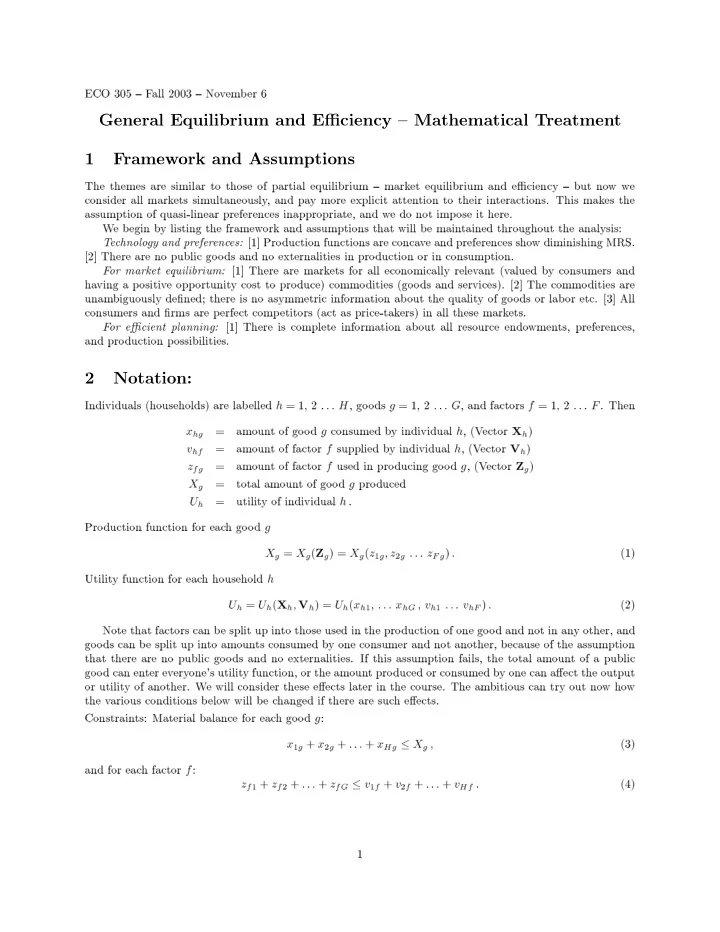
ECO 305 — Fall 2003 — November 6 General Equilibrium and Efficiency — Mathematical Treatment 1 Framework and Assumptions The themes are similar to those of partial equilibrium — market equilibrium and efficiency — but now we consider all markets simultaneously, and pay more explicit attention to their interactions. This makes the assumption of quasi-linear preferences inappropriate, and we do not impose it here. We begin by listing the framework and assumptions that will be maintained throughout the analysis: Technology and preferences: [1] Production functions are concave and preferences show diminishing MRS. [2] There are no public goods and no externalities in production or in consumption. For market equilibrium: [1] There are markets for all economically relevant (valued by consumers and having a positive opportunity cost to produce) commodities (goods and services). [2] The commodities are unambiguously defined; there is no asymmetric information about the quality of goods or labor etc. [3] All consumers and firms are perfect competitors (act as price-takers) in all these markets. For efficient planning: [1] There is complete information about all resource endowments, preferences, and production possibilities. 2 Notation: Individuals (households) are labelled h = 1 , 2 . . . H , goods g = 1 , 2 . . . G , and factors f = 1 , 2 . . . F . Then x hg = amount of good g consumed by individual h , (Vector X h ) v hf = amount of factor f supplied by individual h , (Vector V h ) z fg = amount of factor f used in producing good g , (Vector Z g ) X g = total amount of good g produced U h = utility of individual h . Production function for each good g X g = X g ( Z g ) = X g ( z 1 g , z 2 g . . . z F g ) . (1) Utility function for each household h U h = U h ( X h , V h ) = U h ( x h 1 , . . . x hG , v h 1 . . . v hF ) . (2) Note that factors can be split up into those used in the production of one good and not in any other, and goods can be split up into amounts consumed by one consumer and not another, because of the assumption that there are no public goods and no externalities. If this assumption fails, the total amount of a public good can enter everyone’s utility function, or the amount produced or consumed by one can affect the output or utility of another. We will consider these effects later in the course. The ambitious can try out now how the various conditions below will be changed if there are such effects. Constraints: Material balance for each good g : x 1 g + x 2 g + . . . + x Hg ≤ X g , (3) and for each factor f : z f 1 + z f 2 + . . . + z fG ≤ v 1 f + v 2 f + . . . + v Hf . (4) 1

3 Optimization Suppose a benevolent dictator plans all production and allocation to maximize social welfare W = W ( U 1 , U 2 . . . U H ) (5) subject to the constraints (1), (2), (3) and (4). Substitute out the conditions (1) and (2) that define outputs and utilities. Keep the constraints of material balance, and define Lagrange multipliers α g for the goods balance constraints and β f for the factor balance constraints. Then, omitting arguments of functions for brevity, the Lagrangian is � H G � H � F G � � � � � � L = W + α g X g − x hg + β f v hf − z fg . g =1 h =1 f =1 h =1 g =1 The first-order conditions are: For goods consumption quantities x hg : ∂W ∂U h − α g = 0 . (6) ∂U h ∂x hg For factor supplies v hf : ∂W ∂U h + β f = 0 . (7) ∂U h ∂v hf For factor uses z fg : ∂X g α g − β f = 0 . (8) ∂z fg Note the difference of sign in the conditions for goods’ consumption and factor supplies — this is because goods provide utility and labor supply gives disutility to consumers. If some factors (land) can be supplied without disutility, then their quantities will be set equal to the maximum each consumer possesses, and (7) will be replaced by inequality conditions for a boundary solution. This will not be discussed in any detail here, as it does not raise any important issues for our present purpose. We can rewrite the conditions to bring out their relation to the geometric treatment of November 4. We do this by picking conditions in suitable pairs, and dividing the two equations in each pair: Consumption efficiency: For any two goods, say 1 and 2, ∂U h /∂x h 1 = α 1 , same for all h . ∂U h /∂x h 2 α 2 The left hand side is the marginal rate of substitution between goods 1 and 2 along an indifference curve for household h ; thus the MRS between any fixed pair of goods should be equal for all households. This is the tangency condition for goods allocation in the exchange Edgeworth box of Figure 1 of November 4. Then the right hand side, α 1 /α 2 should play the role of the relative price of the two goods. We will soon see that such is indeed the case. Production efficiency: For any two factors, say 1 and 2, ∂X g /∂z 1 g = β 1 , same for all g . ∂X g /∂z 2 g β 2 The left hand side is the marginal rate of technical substitution between factors 1 and 2 along an isoquant for good g ; thus the RTS should be equal for all goods. This is the tangency condition for factor allocation in the Edgeworth box of Figure 3 of November 4. Then the right hand side, β 1 /β 2 , should play the role of the relative price of the two factors, as indeed it will. 2

Joint efficiency: For any one good g and any one factor f , and for all h − ∂U h /∂v hf = β f = ∂X g . ∂U h /∂x hg α g ∂z fg This says that the marginal extra amount of good g that will induce any consumer to supply another marginal unit of factor f should equal the rate at which the production process can transform factor f into good g . This corresponds to the tangency in Figure 4 from November 4. 4 Equilibrium Let p = ( p g ) be the vector of prices of goods and w = ( w f ) the vector of prices of factors. We specify the behavior of firms first; then households. We suppose that good g is made by just one firm, and define its profit function (this needs concave production functions) F � π g ( p g , w ) = max p g X g ( z 1 g , . . . z F g ) − w f z fg . f =1 Then the output supply and factor demand functions are given by Hotelling’s Lemma: X g = ∂π g /∂p g , z fg = − ∂π g /∂w f . (9) In the present context of perfect competition (price-taking) and no externalities, the assumption of one firm per good is harmless: if several firms are making a good, their profit-maximization is carried out independently and simultaneously, and we can effectively regard them as one firm whose profit function is the sum of those of the actual separate ones (and whose output supply function and factor demand functions are likewise sums). Conversely, multi-product firms can be allowed by making the profit function depend on all the relevant output prices. If I h denotes the income of households other than that derived from their sales of factor services, their budget constraints are G F � � p g x hg ≤ w f v hf + I h . g =1 f =1 Maximizing utility subject to this gives the demand functions x hg = x hg ( p , w , I h ) , v hf = v hf ( p , w , I h ) . (10) Finally, we tie together households’ incomes and firms’ profits. (This is like the “circular flow of income” concept of macroeconomics in ECO 101). Suppose household h owns a fraction θ hg of firm g . Then G � I h = θ hg π g ( p g , w ) . (11) g =1 Equilibrium is defined by the market-clearing conditions for all goods g H � G � � � x hg p , w , θ hg π g ( p g , w ) = X g ( p g , w ) , (12) h =1 g =1 and all factors f G H � G � � � � z fg ( p g , w ) = v hf p , w , θ hg π g ( p g , w ) . (13) g =1 h =1 g =1 Every household and firm makes its decisions accepting the ruling prices ( p g ) and ( w f ), and the prices are determined by the requirement of market-clearing. Thus we are to regard prices as the “unknowns” that are solved from the equilibrium conditions. 3