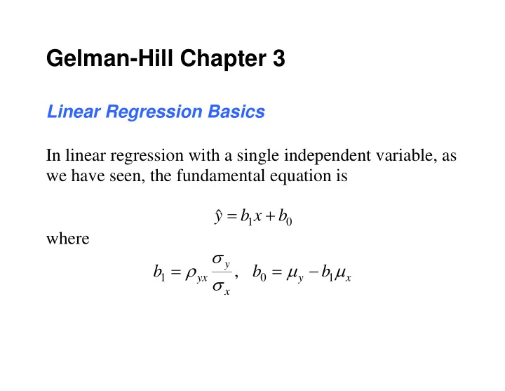
Gelman-Hill Chapter 3 Linear Regression Basics In linear regression - PowerPoint PPT Presentation

Gelman-Hill Chapter 3 Linear Regression Basics In linear regression with a single independent variable, as we have seen, the fundamental equation is   ˆ y b x b 1 0 where        y , b b b 1  0 1 yx y x x

Bivariate Normal Regression A key result is that if y and x have a bivariate normal distribution, then the conditional distribution of y given  is normal, with mean     , and standard x a b a b | 1 0 y x a      2 deviation 1 e xy y Note that the conditional mean is “on the regression line” relating y to x, and the conditional standard deviation is the same for all conditional values of x .

Preliminary Setup Set up a working directory for this lecture, and copy the Chapter 3 files to it. Switch to your working directory, using the Change dir command:

Then make sure you have installed the R package arm . If you are in the micro lab, you will need to tell R to install packages into a personal library directory, because the micro lab prohibits alteration of the basic R library space as a precaution against viruses. To do this, after you have switched to your working directory, create a personal library directory, and tell R to install packages in this directory. For example, create the directory c:/MyRLibs, then issue the R command > .libPaths(‘c:/MyRLibs’) R will now install new packages in this directory.

Next, install the arm package.

Kids Data Example G-H begin with a very simple regression in which one of the predictors is binary. We read in the data with the command > kidiq <- read.dta(file="kidiq.dta") This is actually a “data frame.” Let’s take a look with the editor. > edit(kidsiq)

We can access the objects in a data frame by using the $ character. For example, to compute the mean of the kid_score variable, we could say > mean(kidiq$kid_score) [1] 87 However, it is a lot easier to attach the data frame, after which we can simply refer to the variables by name. > attach(kidiq) > mean(kid_score) [1] 87

G-H have labels in their chapter that are slightly different from those in their data file. To maintain compatibility with the chapter, we create some new variables with these names. > kid.score <-kid_score > mom.hs <- mom_hs > mom.iq <- mom_iq Let’s look at a plot of kid.score versus the mom.hs variable. > plot(mom.hs, kid.score)

140 120 100 kid.score 80 60 40 20 0.0 0.2 0.4 0.6 0.8 1.0 mom.hs Not much of a plot, because mom.hs is binary. To fit a linear model to these variables, we use the lm command, and save the result in a fit object.

> fit.1 <- lm (kid.score ~ mom.hs) The model code kid.score ~ mom.hs is R code for     kid.score mom.hs error b b 1 0 The intercept term is assumed, as is the error. Once we have the fit, we can examine the result in a variety of ways.

> display(fit.1) lm(formula = kid.score ~ mom.hs) coef.est coef.se (Intercept) 77.55 2.06 mom.hs 11.77 2.32 --- n = 434, k = 2 residual sd = 19.85, R-Squared = 0.06

> print(fit.1) Call: lm(formula = kid.score ~ mom.hs) Coefficients: (Intercept) mom.hs 77.5 11.8

> summary(fit.1) Call: lm(formula = kid.score ~ mom.hs) Residuals: Min 1Q Median 3Q Max -57.55 -13.32 2.68 14.68 58.45 Coefficients: Estimate Std. Error t value Pr(>|t|) (Intercept) 77.55 2.06 37.67 <2e-16 *** mom.hs 11.77 2.32 5.07 6e-07 *** --- Signif. codes: 0 ‘***’ 0.001 ‘**’ 0.01 ‘*’ 0.05 ‘.’ 0.1 ‘ ’ 1 Residual standard error: 20 on 432 degrees of freedom Multiple R-squared: 0.0561, Adjusted R-squared: 0.0539 F-statistic: 25.7 on 1 and 432 DF, p-value: 5.96e-07

Plotting the Regression plot (mom.hs, kid.score, xlab="Mother HS", ylab="Child test score") curve (coef(fit.1)[1] + coef(fit.1)[2]*x, add=TRUE) 140 120 100 Child test score 80 60 40 20 0.0 0.2 0.4 0.6 0.8 1.0 Mother HS

> ### two fitted regression lines > > ## model with no interaction > fit.3 <- lm (kid.score ~ mom.hs + mom.iq) > colors <- ifelse (mom.hs==1, "black", "gray") > plot (mom.iq, kid.score, xlab="Mother IQ score", ylab="Child test score", + col=colors, pch=20) > curve (cbind (1, 1, x) %*% coef(fit.3), add=TRUE, col="black") > curve (cbind (1, 0, x) %*% coef(fit.3), add=TRUE, col="gray") 140 120 100 Child test score 80 60 40 20 70 80 90 100 110 120 130 140 Mother IQ score

Interpretation of Coefficients > print(fit.3) Call: lm(formula = kid.score ~ mom.hs + mom.iq) Coefficients: (Intercept) mom.hs mom.iq 25.732 5.950 0.564 “Predictive” vs. “Counterfactual” Interpretation

> ### two fitted regression lines: > ## model with interaction > fit.4 <- lm (kid.score ~ mom.hs + mom.iq + mom.hs:mom.iq) > colors <- ifelse (mom.hs==1, "black", "gray") > plot (mom.iq, kid.score, xlab="Mother IQ score", ylab="Child test score", + col=colors, pch=20) > curve (cbind (1, 1, x, 1*x) %*% coef(fit.4), add=TRUE, col="black") > curve (cbind (1, 0, x, 0*x) %*% coef(fit.4), add=TRUE, col="gray") >print(fit.4) Call: lm(formula = kid.score ~ mom.hs + mom.iq + mom.hs:mom.iq) Coefficients: (Intercept) mom.hs mom.iq mom.hs:mom.iq -11.482 51.268 0.969 -0.484

140 130 120 Mother IQ score 110 100 90 80 70 140 120 100 80 60 40 20 Child test score

The overall equation is         kid.score 51.3 mom.hs .969 mom.iq .484 mom.hs mom.iq 11.5 With mom.hs = 0, the equation becomes     kid.score 11.5 .969 mom.iq With mom.hs = 1, the equation becomes       kid.score 51.3 .969 mom.iq .484 mom.iq 11.5    39.8 .485 mom.iq We can see this better by extending the plot:

> plot (mom.iq, kid.score, xlab="Mother IQ score", ylab="Child test score",col=colors, pch=20,xlim=c(0,150),ylim=c(-15,150)) > curve (cbind (1, 1, x, 1*x) %*% coef(fit.4), add=TRUE, col="black") > curve (cbind (1, 0, x, 0*x) %*% coef(fit.4), add=TRUE, col="gray")