g ( x ) := E [ Y | X = x ] := yPr [ Y = y | X = x ] . Recall that L - PowerPoint PPT Presentation

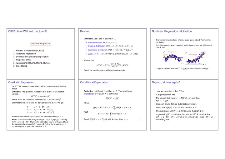
CS70: Jean Walrand: Lecture 31. Review Nonlinear Regression: Motivation Definitions Let X and Y be RVs on Ω . There are many situations where a good guess about Y given X is not linear. ◮ Joint Distribution: Pr [ X = x , Y = y ] Nonlinear Regression E.g., (diameter of object, weight), (school years, income), (PSA level, ◮ Marginal Distribution: Pr [ X = x ] = ∑ y Pr [ X = x , Y = y ] cancer risk). ◮ Conditional Distribution: Pr [ Y = y | X = x ] = Pr [ X = x , Y = y ] 1. Review: joint distribution, LLSE Pr [ X = x ] ◮ LLSE: L [ Y | X ] = a + bX where a , b minimize E [( Y − a − bX ) 2 ] . 2. Quadratic Regression 3. Definition of Conditional expectation 4. Properties of CE We saw that 5. Applications: Diluting, Mixing, Rumors L [ Y | X ] = E [ Y ]+ cov ( X , Y ) ( X − E [ X ]) . 6. CE = MMSE var [ X ] Our goal: explore estimates ˆ Y = g ( X ) for nonlinear functions g ( · ) . Recall the non-Bayesian and Bayesian viewpoints. Quadratic Regression Conditional Expectation Deja vu, all over again? Let X , Y be two random variables defined on the same probability space. Have we seen this before? Yes. Definition Let X and Y be RVs on Ω . The conditional Definition: The quadratic regression of Y over X is the random expectation of Y given X is defined as variable Is anything new? Yes. Q [ Y | X ] = a + bX + cX 2 The idea of defining g ( x ) = E [ Y | X = x ] and then E [ Y | X ] = g ( X ) where a , b , c are chosen to minimize E [( Y − a − bX − cX 2 ) 2 ] . E [ Y | X ] = g ( X ) . Derivation: We set to zero the derivatives w.r.t. a , b , c . We get where Big deal? Quite! Simple but most convenient. E [ Y − a − bX − cX 2 ] 0 = g ( x ) := E [ Y | X = x ] := ∑ yPr [ Y = y | X = x ] . Recall that L [ Y | X ] = a + bX is a function of X . E [( Y − a − bX − cX 2 ) X ] 0 = y This is similar: E [ Y | X ] = g ( X ) for some function g ( · ) . Fact E [( Y − a − bX − cX 2 ) X 2 ] 0 = E [ Y | X = x ] = ∑ Y ( ω ) Pr [ ω | X = x ] . In general, g ( X ) is not linear, i.e., not a + bX . It could be that ω We solve these three equations in the three unknowns ( a , b , c ) . g ( X ) = a + bX + cX 2 . Or that g ( X ) = 2sin ( 4 X )+ exp {− 3 X } . Or Proof: E [ Y | X = x ] = E [ Y | A ] with A = { ω : X ( ω ) = x } . something else. Note: These equations imply that E [( Y − Q [ Y | X ]) h ( X )] = 0 for any h ( X ) = d + eX + fX 2 . That is, the estimation error is orthogonal to all the quadratic functions of X . Hence, Q [ Y | X ] is the projection of Y onto the space of quadratic functions of X .

Properties of CE Properties of CE Properties of CE E [ Y | X = x ] = ∑ E [ Y | X = x ] = ∑ yPr [ Y = y | X = x ] yPr [ Y = y | X = x ] y y E [ Y | X = x ] = ∑ Theorem yPr [ Y = y | X = x ] Theorem (a) X , Y independent ⇒ E [ Y | X ] = E [ Y ] ; y (a) X , Y independent ⇒ E [ Y | X ] = E [ Y ] ; (b) E [ aY + bZ | X ] = aE [ Y | X ]+ bE [ Z | X ] ; Theorem (c) E [ Yh ( X ) | X ] = h ( X ) E [ Y | X ] , ∀ h ( · ) ; (b) E [ aY + bZ | X ] = aE [ Y | X ]+ bE [ Z | X ] ; (a) X , Y independent ⇒ E [ Y | X ] = E [ Y ] ; (d) E [ h ( X ) E [ Y | X ]] = E [ h ( X ) Y ] , ∀ h ( · ) ; (b) E [ aY + bZ | X ] = aE [ Y | X ]+ bE [ Z | X ] ; (c) E [ Yh ( X ) | X ] = h ( X ) E [ Y | X ] , ∀ h ( · ) ; (e) E [ E [ Y | X ]] = E [ Y ] . (c) E [ Yh ( X ) | X ] = h ( X ) E [ Y | X ] , ∀ h ( · ) ; (d) E [ h ( X ) E [ Y | X ]] = E [ h ( X ) Y ] , ∀ h ( · ) ; (d) E [ h ( X ) E [ Y | X ]] = E [ h ( X ) Y ] , ∀ h ( · ) ; Proof: (continued) (e) E [ E [ Y | X ]] = E [ Y ] . (e) E [ E [ Y | X ]] = E [ Y ] . (d) E [ h ( X ) E [ Y | X ]] = ∑ h ( x ) E [ Y | X = x ] Pr [ X = x ] Proof: x Proof: (continued) = ∑ h ( x ) ∑ yPr [ Y = y | X = x ] Pr [ X = x ] (a),(b) Obvious (e) Let h ( X ) = 1 in (d). x y (c) E [ Yh ( X ) | X = x ] = ∑ Y ( ω ) h ( X ( ω ) Pr [ ω | X = x ] = ∑ h ( x ) ∑ yPr [ X = x , y = y ] ω = ∑ x y Y ( ω ) h ( x ) Pr [ ω | X = x ] = h ( x ) E [ Y | X = x ] = ∑ h ( x ) yPr [ X = x , y = y ] = E [ h ( X ) Y ] . ω x , y Properties of CE Application: Calculating E [ Y | X ] Application: Diluting Theorem Let X , Y , Z be i.i.d. with mean 0 and variance 1. We want to (a) X , Y independent ⇒ E [ Y | X ] = E [ Y ] ; calculate (b) E [ aY + bZ | X ] = aE [ Y | X ]+ bE [ Z | X ] ; E [ 2 + 5 X + 7 XY + 11 X 2 + 13 X 3 Z 2 | X ] . (c) E [ Yh ( X ) | X ] = h ( X ) E [ Y | X ] , ∀ h ( · ) ; (d) E [ h ( X ) E [ Y | X ]] = E [ h ( X ) Y ] , ∀ h ( · ) ; (e) E [ E [ Y | X ]] = E [ Y ] . At each step, pick a ball from a well-mixed urn. Replace it with a blue We find ball. Let X n be the number of red balls in the urn at step n . What is Note that (d) says that E [ X n ] ? E [ 2 + 5 X + 7 XY + 11 X 2 + 13 X 3 Z 2 | X ] = 2 + 5 X + 7 XE [ Y | X ]+ 11 X 2 + 13 X 3 E [ Z 2 | X ] Given X n = m , X n + 1 = m − 1 w.p. m / N (if you pick a red ball) and E [( Y − E [ Y | X ]) h ( X )] = 0 . X n + 1 = m otherwise. Hence, = 2 + 5 X + 7 XE [ Y ]+ 11 X 2 + 13 X 3 E [ Z 2 ] E [ X n + 1 | X n = m ] = m − ( m / N ) = m ( N − 1 ) / N = X n ρ , We say that the estimation error Y − E [ Y | X ] is orthogonal to = 2 + 5 X + 11 X 2 + 13 X 3 ( var [ Z ]+ E [ Z ] 2 ) every function h ( X ) of X . with ρ := ( N − 1 ) / N . Consequently, = 2 + 5 X + 11 X 2 + 13 X 3 . E [ X n + 1 ] = E [ E [ X n + 1 | X n ]] = ρ E [ X n ] , n ≥ 1 . We call this the projection property. More about this later. ⇒ E [ X n ] = ρ n − 1 E [ X 1 ] = N ( N − 1 ) n − 1 , n ≥ 1 . = N

Diluting Diluting Application: Mixing Here is a plot: By analyzing E [ X n + 1 | X n ] , we found that E [ X n ] = N ( N − 1 N ) n − 1 , n ≥ 1 . Here is another argument for that result. Consider one particular red ball, say ball k . At each step, it remains red w.p. ( N − 1 ) / N , when another ball is picked. Thus, the probability that it is still red at step n is [( N − 1 ) / N ] n − 1 . Let At each step, pick a ball from each well-mixed urn. We transfer them Y n ( k ) = 1 { ball k is red at step n } . to the other urn. Let X n be the number of red balls in the bottom urn at step n . What is E [ X n ] ? Then, X n = Y n ( 1 )+ ··· + Y n ( N ) . Hence, Given X n = m , X n + 1 = m + 1 w.p. p and X n + 1 = m − 1 w.p. q where p = ( 1 − m / N ) 2 (B goes up, R down) and q = ( m / N ) 2 (R goes E [ X n ] = E [ Y n ( 1 )+ ··· + Y n ( N )] = NE [ Y n ( 1 )] NPr [ Y n ( 1 ) = 1 ] = N [( N − 1 ) / N ] n − 1 . up, B down). = Thus, E [ X n + 1 | X n ] = X n + p − q = X n + 1 − 2 X n / N = 1 + ρ X n , ρ := ( 1 − 2 / N ) . Mixing Application: Mixing Application: Going Viral Consider a social network (e.g., Twitter). Here is the plot. You start a rumor (e.g., Walrand is really weird). We saw that E [ X n + 1 | X n ] = 1 + ρ X n , ρ := ( 1 − 2 / N ) . Hence, You have d friends. Each of your friend retweets w.p. p . Each of your friends has d friends, etc. E [ X n + 1 ] = 1 + ρ E [ X n ] E [ X 2 ] = 1 + ρ N ; E [ X 3 ] = 1 + ρ ( 1 + ρ N ) = 1 + ρ + ρ 2 N Does the rumor spread? Does it die out (mercifully)? E [ X 4 ] = 1 + ρ ( 1 + ρ + ρ 2 N ) = 1 + ρ + ρ 2 + ρ 3 N E [ X n ] = 1 + ρ + ··· + ρ n − 2 + ρ n − 1 N . Hence, E [ X n ] = 1 − ρ n − 1 + ρ n − 1 N , n ≥ 1 . 1 − ρ In this example, d = 4.

Application: Going Viral Application: Going Viral Application: Wald’s Identity Here is an extension of an identity we used in the last slide. Theorem Wald’s Identity Assume that X 1 , X 2 ,... and Z are independent, where Z takes values in { 0 , 1 , 2 ,... } An easy extension: Assume that everyone has an independent and E [ X n ] = µ for all n ≥ 1. number D i of friends with E [ D i ] = d . Then, the same fact holds. Then, Fact: Let X = ∑ ∞ n = 1 X n . Then, E [ X ] < ∞ iff pd < 1 . To see this, note that given X n = k , and given the numbers of friends E [ X 1 + ··· + X Z ] = µ E [ Z ] . D 1 = d 1 ,..., D k = d k of these X n people, one has Proof: X n + 1 = B ( d 1 + ··· + d k , p ) . Hence, Given X n = k , X n + 1 = B ( kd , p ) . Hence, E [ X n + 1 | X n = k ] = kpd . Proof: Thus, E [ X n + 1 | X n ] = pdX n . Consequently, E [ X n ] = ( pd ) n − 1 , n ≥ 1 . E [ X n + 1 | X n = k , D 1 = d 1 ,..., D k = d k ] = p ( d 1 + ··· + d k ) . E [ X 1 + ··· + X Z | Z = k ] = µ k . If pd < 1, then E [ X 1 + ··· + X n ] ≤ ( 1 − pd ) − 1 = ⇒ E [ X ] ≤ ( 1 − pd ) − 1 . Thus, E [ X n + 1 | X n = k , D 1 ,..., D k ] = p ( D 1 + ··· + D k ) . Thus, E [ X 1 + ··· + X Z | Z ] = µ Z . If pd ≥ 1, then for all C one can find n s.t. Consequently, E [ X n + 1 | X n = k ] = E [ p ( D 1 + ··· + D k )] = pdk . E [ X ] ≥ E [ X 1 + ··· + X n ] ≥ C . Hence, E [ X 1 + ··· + X Z ] = E [ µ Z ] = µ E [ Z ] . Finally, E [ X n + 1 | X n ] = pdX n , and E [ X n + 1 ] = pdE [ X n ] . In fact, one can show that pd ≥ 1 = ⇒ Pr [ X = ∞ ] > 0. We conclude as before. CE = MMSE CE = MMSE E [ Y | X ] and L [ Y | X ] as projections Theorem Theorem CE = MMSE E [ Y | X ] is the ‘best’ guess about Y based on X . g ( X ) := E [ Y | X ] is the function of X that minimizes Specifically, it is the function g ( X ) of X that E [( Y − g ( X )) 2 ] . minimizes E [( Y − g ( X )) 2 ] . Proof: Let h ( X ) be any function of X . Then E [( Y − h ( X )) 2 ] E [( Y − g ( X )+ g ( X ) − h ( X )) 2 ] = E [( Y − g ( X )) 2 ]+ E [( g ( X ) − h ( X )) 2 ] = + 2 E [( Y − g ( X ))( g ( X ) − h ( X ))] . But, E [( Y − g ( X ))( g ( X ) − h ( X ))] = 0 by the projection property . L [ Y | X ] is the projection of Y on { a + bX , a , b ∈ ℜ } : LLSE Thus, E [( Y − h ( X )) 2 ] ≥ E [( Y − g ( X )) 2 ] . E [ Y | X ] is the projection of Y on { g ( X ) , g ( · ) : ℜ → ℜ } : MMSE.