Functional Equations & Neural Networks for Time Series - PowerPoint PPT Presentation
Functional Equations & Neural Networks for Time Series Interpolation Lars Kindermann, AWI Achim Lewandowski, OEFAI An old experiment v 0 v 1 Drop an object with different speeds and measure the speed at the ground Data v 0 x 0 v 1 free
Functional Equations & Neural Networks for Time Series Interpolation Lars Kindermann, AWI Achim Lewandowski, OEFAI
An old experiment v 0 v 1 Drop an object with different speeds and measure the speed at the ground Data v 0 x 0 v 1 free fall x m v m = ? friction x 1 v 1 = f v 0 v 0 Question: What’s the speed v m after half the way at x m ?
Solving with traditional Physics Free Fall: 2 x Theory: = g t 2 2 Model: v 1 = f v 0 = v 0 + 2g x with data fitted g With additional Friction : 2 x x 2 x x Theory: = g – k 1 – k 2 – f t t 2 t t Model: Integrate numerically and fit and - already a non-trivial Problem! g k
A Data-based Aproach Theory: Assume translation invariance v 0 v 0 x 0 x 0 x m v m divide into v m = two equal steps... x 1 x 1 v m v 0 v 1 = = v 1 v 1 = f v 0 v = f v and solve this functional equation for
A Functional Equation x = f x A solution of this equation is a kind of square root of the function . f n n • I x If : is a function , we look for another function which f x R I R f x composed with itself equals : = f x f 2 x Because the self-composition of a function f f x = is also called “iteration”, the square root of a function is usually called its iterative root. n x f m x = is solved by the fractional iterates of a function : f f m n x = x
A Functional Equation x = f x A solution of this equation is called a square root of . f n n • I x If f x : R I R is a function , we look for another function which f x composed with itself equals : = f x f 2 x Because the self-composition of a function f f x = is also called “iteration”, the square root of a function is usually called its iterative root. x y f = x y n x f m x is solved by the fractional iterates of a function : f = x y f = f m n x = x x y 3 - - - 5 f
Generalized Iteration f n x The exponential notation of the iteration of functions can be extended beyond integer exponents: f 1 • means f f n • for positive integers are the well known iterations of n f f 0 x f 0 • denotes the identity function, = x – 1 • f is the inverse funktion of f – n • f is the -th iteration of the inverse of n f f 1 n • is the -th iterative root of n f f m n • is the -th iteration of the -th iterative root or fractional iterate of m n f f t x The family forms the continuous iteration group of . f f a f b x f a + b Within this the translation equation is satisfied. x =
Map this to a Network share weights f x x x f x x n m 1 loop n times f x x f m n = f 1 n f
Training Methods • Weight Copy: Train only the last layer and copy the weights continously backwards • Weight Sharing: Initialize corresponding weights with equal values and sum up all w i delivered by the network learning rule • Weight Coupling: Start with different values and let the corresponding weights of the iteration layers approach each other by a term like w j w i = – w i • Regularization: Add a penalty term to the error function which assigns an error to the weight-differences to regularize the network. This allows to uti- lize second order gradient methods like quasi Newton for faster training. • Exact Gradient: Compute the exact gradients for an iterated Network
Results for „The Fall“ no friction with friction 10 10 9 9 measurement for v1 (training data) physics for vm (prediction task) fractional iterates (network results) f 1 4 8 8 v 1 = f v 0 7 f 0 v 0 7 f 1 2 v m = v 0 = v 0 End Velocity [m/s] End Velocity [m/s] 6 6 f 0 v 0 f 3 4 = v 0 5 5 f 3 4 4 4 f 1 2 v 1 = f v 0 v m = v 0 3 3 f 1 4 2 2 measurement for v1 (training data) physics for vm (prediction task) 1 1 fractional iterates (network results) 0 0 0 1 2 3 4 5 6 7 8 9 10 0 1 2 3 4 5 6 7 8 9 10 Start Velocity [m/s] Start Velocity [m/s] The Network results are conform to the laws of physics up to a mean error of 10 -6
The Embedding Problem v=f(v 0 ,h) 12 Training Data 10 8 v [m/s] 6 v(h) 4 2 0 10 9 8 1.2 7 1 6 5 0.8 4 0.6 trajectories iterative roots 3 0.4 2 v 0 0.2 1 h 0 0 v0 [m/s] h [m]
The Schröder Equation f x c x = One of the most important functional equations: The Eigenvalue problem of functional calculus. 1 – c x Transform to: f x = invert train c f x x x 1 – f
Commuting Functions f x f x = f f x x weight outputs sharing targets f x x f x
Steel Mill Model p 1 p 2 p N pi =set of parameters like force, heat, strip thikness and width... x in x out x 1 x 2 Measuring instrument f x in p 1 , f x 1 p 2 , f x N , p N – 1 F x in p 1 p N , - The steel bands are processed by N identical stands in a row - x in p i x out , are known and can be measured - p 2 ... p N x out = F x in p 1 ...p N = f ...f f x in p 1 ,
Steel Mill Network
Timeseries Interpolation n For a given autoregressive Box-Jenkins AR(n) timeseries , we x t = a k x t – k k = 1 F R n R n define the function : which maps the vector of the last n samples x t = x t one step into the future x t = x t as x t x t x t – 1 – 1 – n – 1 – n – 1 a 1 a 2 a n 1 0 0 0 F = and can simply write x t = F x t now. – 1 0 1 0 0 0 0 1 0 The discrete time evolution of the the system can be calculated using the F n x t matrix powers of F: . x t = + n – 1
Using Generalized Matrix Powers F t This autoregressive system is called linear embeddable if the matrix power R + exists also for all real t . This is the case if can be decomposed into F S A S 1 – i with being a diagonal matrix consisting of the eigenvalues F = A of and being an invertible square matrix which columns are the eigenvec- F S i tors of . Additionally all must be non-negative to have a linear and real F embedding, otherwise we will get a complex embedding. t 0 1 0 S A t S 1 F t – A t Then we can obtain = with = 0 0 t 0 n 0 F t x 0 Now we have a continuous function and the interpolation of the x t = original time series x t consists of the first element of . x
Example: A continuous Fibonacci Function The Fibonacci series x 0 = 0 , x 1 = 1 , x t = x t + x t is generated by – 1 – 2 1 1 F = and x 1 = 1 0 . By eigenvalue decomposition of we get F 1 0 1 1 - 1 - - t - - - - - - - - - - - - 0 1 + 5 - 1 – 5 1 + 5 - - - - - - - - - - - - - - - - - - – – x 1 - - - - - - - - - - - - - - - - - - - - - - - - - - - - - - - - - - - - - - - - - - - - - - - 5 2 1 F t x 1 SA t S 1 2 5 2 x t = = = 2 2 + 1 1 0 t 1 1 1 1 0 1 – 5 - - - + - - - - - - - - - - - - - - - - - - - - - - - - - - - - - - - - - - 2 - - - - - - - - - - - - – 2 2 5 5 t t 1 1 + 5 1 – 5 - - - - - - - - - - - - - - - - - - - - - - - - - - - - - - - - - - - - - - - That is Binet’s formula in the first component x t = – 2 2 5
Nonlinear Example A time series of yearly snapshots from a discrete non linear Lotka-Volterra type predator - prey system ( x = hare, y = lynx) is used as training data: x t y t x t = 1 + a – b y t and y t = 1 – c + d x t + 1 + 1 7 From these samples we calculate the monthly population by use of 6 a neural network based method 5 to compute iterative roots and fractional iterates. 4 Predator The given method provides a 3 natural way to estimate not only the values over a year, but also to 2 extrapolate arbitrarily smooth into 1 the future. 0 0 2 4 6 8 10 12 Prey
Recommend


More recommend
Explore More Topics
Stay informed with curated content and fresh updates.