From an Interval to a Natural What We Do: . . . Extreme - PowerPoint PPT Presentation

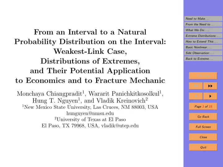
Need to Make . . . From the Need to . . . From an Interval to a Natural What We Do: . . . Extreme Distributions: . . . Probability Distribution on the Interval: How to Extend This . . . Basic Nonlinear . . . Weakest-Link Case, Side Observation: . . . Back to Extreme . . . Distributions of Extremes, and Their Potential Application Title Page to Economics and to Fracture Mechanic ◭◭ ◮◮ Monchaya Chiangpradit 1 , Wararit Panichkitkosolkul 1 , ◭ ◮ Hung T. Nguyen 1 , and Vladik Kreinovich 2 1 New Mexico State University, Las Cruces, NM 88003, USA Page 1 of 15 hunguyen@nmsu.edu Go Back 2 University of Texas at El Paso El Paso, TX 79968, USA, vladik@utep.edu Full Screen Close Quit

Need to Make . . . 1. Need to Make Decisions under Interval Uncertainty From the Need to . . . • One of the main practical objectives is to make deci- What We Do: . . . sions. Extreme Distributions: . . . How to Extend This . . . • Decisions are usually made on the utility values u ( a ) Basic Nonlinear . . . of different alternatives a . Side Observation: . . . • Under interval uncertainty, we only know the interval Back to Extreme . . . u ( a ) = [ u ( a ) , u ( a )] containing u ( a ). Title Page • When two intervals intersect u ( a ) ∩ u ( b ) � = ∅ , in prin- ◭◭ ◮◮ ciple, each of the two alternatives can be better. ◭ ◮ • Intuitively, it is sometimes clear that a is “more prob- Page 2 of 15 able” to be better than b . Go Back • Example: if u ( a ) = [0 , 1 . 1] and u ( b ) = [0 . 9 , 2], the b is most probably better. Full Screen Close Quit

Need to Make . . . 2. From the Need to Make Decisions to the Need to From the Need to . . . Assign Probabilities What We Do: . . . • Reminder: in situations with interval uncertainty, we Extreme Distributions: . . . need to make decisions. How to Extend This . . . Basic Nonlinear . . . • According to decision theory: Side Observation: . . . – a consistent decision making procedure under un- Back to Extreme . . . certainty Title Page is equivalent to ◭◭ ◮◮ – assigning “subjective” probabilities to different val- ◭ ◮ ues within each uncertainty domain. Page 3 of 15 • In our case: uncertainty domain is an interval. Go Back • Conclusion: we need a natural way to assign probabil- Full Screen ities on an interval. Close Quit

Need to Make . . . 3. What We Do: Consider Weakest Link Case From the Need to . . . • General problem: assigning probabilities on an interval. What We Do: . . . Extreme Distributions: . . . • What we do: consider a practically important case of How to Extend This . . . the “weakest link” arrangement. Basic Nonlinear . . . • What it means: the collapse of each link is catastrophic Side Observation: . . . for a system. Back to Extreme . . . • Example 1: fracture mechanics, when a fracture in one Title Page of the areas makes the whole plane inoperable. ◭◭ ◮◮ • Example 2: economics, when the collapse of one large ◭ ◮ bank or one country can have catastrophic consequences. Page 4 of 15 • General feature: the quality of a system is determined Go Back by the smallest (min v i ) of the corresponding values v i . i Full Screen • In mathematical terms: the distribution of min v i is i Close called the distribution of extremes . Quit

Need to Make . . . 4. Extreme Distributions: Standard Theory From the Need to . . . • We want to find: G ( v 0 ) = 1 − F ( v 0 ) = Prob( v > v 0 ), What We Do: . . . where F ( v 0 ) is a cumulative distribution function. Extreme Distributions: . . . How to Extend This . . . • Fact: the numerical value of a physical quantity v de- Basic Nonlinear . . . pends: Side Observation: . . . – on the choice of a measuring unit v → a · v Back to Extreme . . . (e.g., 1.7 m = 170 cm), and Title Page – on the choice of the starting point v → v + b ◭◭ ◮◮ (e.g.: A.D. or since the French Revolution). ◭ ◮ • Conclusion: we want to find a family G of distributions { G ( a · v 0 + b ) } a,b . Page 5 of 15 • Fact: v ′ def Go Back = min v i > v 0 ⇔ v 1 > v 0 & . . . & v n > v 0 , so Full Screen n G ′ ( v 0 ) = Prob( v > v 0 ) = � Prob( v i > v 0 ) = ( G ( v 0 )) n . Close i =1 Quit

Need to Make . . . 5. Extreme Distributions: Standard Derivation From the Need to . . . • Reminder: G ′ ( v 0 ) = ( G i ( v 0 )) n . What We Do: . . . for maximum v ′′ of α · n values, we get Extreme Distributions: . . . • Similarly: G ′′ ( v 0 ) = ( G ( v 0 )) α · n , hence G ′′ ( v 0 ) = ( G ′ ( v 0 )) α . How to Extend This . . . Basic Nonlinear . . . • In the limit: we conclude that if G ( v 0 ) ∈ G , then Side Observation: . . . G α ( v 0 ) ∈ G for all α . Back to Extreme . . . • Thus: for every α , there exist a ( α ) and b ( α ) s.t. Title Page G α ( v 0 ) = G ( a ( α ) · v 0 + b ( α )) . ◭◭ ◮◮ def • Simplification: for g ( v 0 ) = − ln( G ( v 0 )), we get ◭ ◮ α · g ( v 0 ) = g ( a ( α ) · v 0 + b ( α )) . Page 6 of 15 Go Back • Degenerate case: α = 1, a ( α ) = 1, and b ( α ) = 0. Full Screen • Differentiating both sides by α and taking α = 1, we get g = dg · ( a · v 0 + b ), i.e., dg dv 0 Close def = a ′ (1)). g = a · v 0 + b ( a dv 0 Quit

Need to Make . . . 6. Extreme Distributions: Derivation (cont-d) From the Need to . . . • Reminder: dg dv 0 What We Do: . . . g = a · v 0 + b. Extreme Distributions: . . . • When a = 0 : integration leads to ln( g ) = v 0 How to Extend This . . . b + c , so Basic Nonlinear . . . � v 0 � g ( v 0 ) = exp b + c . Side Observation: . . . Back to Extreme . . . � v 0 � �� • Conclusion: G ( v 0 ) = exp − exp b + c . Title Page def • When a � = 0 : for v = v 0 + ∆ v , with ∆ v = b/a , we get ◭◭ ◮◮ dg g = dv a · v hence ln( g ) = a · ln( v ) + c . ◭ ◮ Page 7 of 15 • Conclusion: g = c · v a = c · ( v 0 − ∆ v ) a , hence Go Back G ( v 0 ) = exp ( − c · ( v 0 − ∆ v ) a ) . Full Screen • Comment. We get two different types of distributions Close depending on whether a > 0 or a < 0. Quit

Need to Make . . . 7. How to Extend This Analysis to Distributions on From the Need to . . . an Interval: Discussion What We Do: . . . • Symmetries: the above derivations were based on the Extreme Distributions: . . . assumption that we have linear symmetries How to Extend This . . . Basic Nonlinear . . . v 0 → a · v 0 + b. Side Observation: . . . • Examples: Back to Extreme . . . Title Page – sometimes, we only have scale-invariance – 0 is fixed (height); ◭◭ ◮◮ – sometimes, we also have shift-invariance (tempera- ◭ ◮ ture, time). Page 8 of 15 • Problem: the only linear transformation that preserves Go Back the interval is identity. Full Screen • Our solution: go beyond linear symmetries, to more Close general (non-linear) symmetries. Quit

Need to Make . . . 8. Basic Nonlinear Symmetries From the Need to . . . • Sometimes, a system also has nonlinear symmetries. What We Do: . . . Extreme Distributions: . . . • If a system is invariant under f and g , then: How to Extend This . . . – it is invariant under their composition f ◦ g , and Basic Nonlinear . . . – it is invariant under the inverse transformation f − 1 . Side Observation: . . . • In mathematical terms, this means that symmetries Back to Extreme . . . form a group . Title Page • In practice, at any given moment of time, we can only ◭◭ ◮◮ store and describe finitely many parameters. ◭ ◮ • Thus, it is reasonable to restrict ourselves to finite- Page 9 of 15 dimensional groups. Go Back • Question (N. Wiener): describe all finite-dimensional Full Screen groups that contain all linear transformations. Close • Answer (for real numbers): all elements of this group are fractionally-linear x → ( a · x + b ) / ( c · x + d ) . Quit

Need to Make . . . 9. Side Observation: Symmetries Explain the Basic From the Need to . . . Formulas of Neural Networks What We Do: . . . • What needs explaining: formula for the activation func- Extreme Distributions: . . . tion f ( x ) = 1 / (1 + e − x ). How to Extend This . . . Basic Nonlinear . . . • A change in the input starting point: x → x + s . Side Observation: . . . • Reasonable requirement: the new output f ( x + s ) equiv- Back to Extreme . . . alent to the f ( x ) mod. appropriate transformation. Title Page • Reminder: all appropriate transformations are frac- ◭◭ ◮◮ tionally linear. ◭ ◮ • Conclusion: f ( x + s ) = a ( s ) · f ( x ) + b ( s ) c ( s ) · f ( x ) + d ( s ) . Page 10 of 15 • Differentiating both sides by s and equating s to 0, we Go Back get a differential equation for f ( x ). Full Screen • Its known solution is the above activation function – Close which can thus be explained by symmetries. Quit