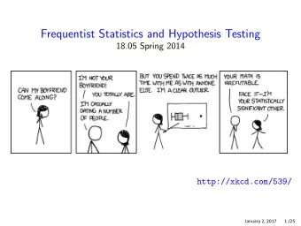
Frequentist Statistics DS GA 1002 Probability and Statistics for - PowerPoint PPT Presentation

Approximate confidence interval for the mean P ( µ ∈ I n ) � �� � �� √ nQ − 1 � α √ nQ − 1 � α Y n > µ + S n Y n < µ − S n = 1 − P − P 2 2

Approximate confidence interval for the mean P ( µ ∈ I n ) � �� � �� √ nQ − 1 � α √ nQ − 1 � α Y n > µ + S n Y n < µ − S n = 1 − P − P 2 2 � √ n ( Y n − µ ) �� � √ n ( Y n − µ ) �� > Q − 1 � α < − Q − 1 � α = 1 − P − P S n 2 S n 2

Approximate confidence interval for the mean P ( µ ∈ I n ) � �� � �� √ nQ − 1 � α √ nQ − 1 � α Y n > µ + S n Y n < µ − S n = 1 − P − P 2 2 � √ n ( Y n − µ ) �� � √ n ( Y n − µ ) �� > Q − 1 � α < − Q − 1 � α = 1 − P − P S n 2 S n 2 � Q − 1 � α �� ≈ 1 − 2 Q 2

Approximate confidence interval for the mean P ( µ ∈ I n ) � �� � �� √ nQ − 1 � α √ nQ − 1 � α Y n > µ + S n Y n < µ − S n = 1 − P − P 2 2 � √ n ( Y n − µ ) �� � √ n ( Y n − µ ) �� > Q − 1 � α < − Q − 1 � α = 1 − P − P S n 2 S n 2 � Q − 1 � α �� ≈ 1 − 2 Q 2 = 1 − α

Bears in Yosemite Empirical standard deviation is 100 lbs Given that Q ( 1 . 95 ) ≈ 0 . 025, � �� √ nQ − 1 � α � √ nQ − 1 � α Y − σ , Y + σ ≈ [ 188 . 8 , 211 . 3 ] 2 2 is an approximate 95% confidence interval

Interpreting confidence intervals The average weight is between 188.8 and 211.3 lbs with probability 0.95

Interpreting confidence intervals If we repeat the process of sampling the population and computing the confidence interval, then the true value will lie in the interval 95% of the time

Estimating the average height We compute 40 confidence intervals of the form � �� √ nQ − 1 � α � √ nQ − 1 � α Y n − S n , Y n + S n I n := 2 2 � � X ( 1 ) , � � X ( 2 ) , . . . , � Y n := av X ( n ) � � X ( 1 ) , � � X ( 2 ) , . . . , � S n := std X ( n ) for 1 − α = 0 . 95 and different values of n

Estimating the average height: n = 50 True mean

Estimating the average height: n = 200 True mean

Estimating the average height: n = 1000 True mean

Independent identically-distributed sampling Mean-square error Consistency Confidence intervals Nonparametric model estimation Parametric estimation

Nonparametric methods Aim: Estimate the distribution underlying the data Very challenging: many (infinite!) different distributions could have generated the measurements

Empirical cdf The empirical cdf corresponding to data x 1 , . . . , x n is n � F n ( x ) := 1 � 1 x i ≤ x , x ∈ R n i = 1 If data are iid with cdf F X , � F n ( x ) is an unbiased and consistent estimator

Empirical cdf is unbiased � � � F n ( x ) E

Empirical cdf is unbiased � � � � n � 1 � F n ( x ) = E 1 � E X ( i ) ≤ x n i = 1

Empirical cdf is unbiased � � � � n � 1 � F n ( x ) = E 1 � E X ( i ) ≤ x n i = 1 � � n � = 1 1 � E X ( i ) ≤ x n i = 1

Empirical cdf is unbiased � � � � n � 1 � F n ( x ) = E 1 � E X ( i ) ≤ x n i = 1 � � n � = 1 1 � E X ( i ) ≤ x n i = 1 � � � n = 1 � X ( i ) ≤ x P n i = 1

Empirical cdf is unbiased � � � � n � 1 � F n ( x ) = E 1 � E X ( i ) ≤ x n i = 1 � � n � = 1 1 � E X ( i ) ≤ x n i = 1 � � � n = 1 � X ( i ) ≤ x P n i = 1 = F X ( x )

Empirical cdf is consistent The mean square of the empirical cdf is � � � F 2 n ( x ) E

Empirical cdf is consistent The mean square of the empirical cdf is � � � F 2 n ( x ) E   � n � n  1  = E 1 � X ( i ) ≤ x 1 � X ( j ) ≤ x n 2 i = 1 j = 1

Empirical cdf is consistent The mean square of the empirical cdf is � � � F 2 n ( x ) E   � n � n  1  = E 1 � X ( i ) ≤ x 1 � X ( j ) ≤ x n 2 i = 1 j = 1 � � � � n n n � � � = 1 + 1 1 � 1 � X ( i ) ≤ x 1 � E E X ( i ) ≤ x X ( j ) ≤ x n 2 n 2 i = 1 i = 1 j = 1 , i � = j

Empirical cdf is consistent The mean square of the empirical cdf is � � � F 2 n ( x ) E   � n � n  1  = E 1 � X ( i ) ≤ x 1 � X ( j ) ≤ x n 2 i = 1 j = 1 � � � � n n n � � � = 1 + 1 1 � 1 � X ( i ) ≤ x 1 � E E X ( i ) ≤ x X ( j ) ≤ x n 2 n 2 i = 1 i = 1 j = 1 , i � = j � � � � � � n n n � � � = 1 + 1 � � � X ( i ) ≤ x X ( i ) ≤ x X ( j ) ≤ x P P P n 2 n 2 i = 1 i = 1 j = 1 , i � = j

Empirical cdf is consistent The mean square of the empirical cdf is � � � F 2 n ( x ) E   � n � n  1  = E 1 � X ( i ) ≤ x 1 � X ( j ) ≤ x n 2 i = 1 j = 1 � � � � n n n � � � = 1 + 1 1 � 1 � X ( i ) ≤ x 1 � E E X ( i ) ≤ x X ( j ) ≤ x n 2 n 2 i = 1 i = 1 j = 1 , i � = j � � � � � � n n n � � � = 1 + 1 � � � X ( i ) ≤ x X ( i ) ≤ x X ( j ) ≤ x P P P n 2 n 2 i = 1 i = 1 j = 1 , i � = j n n � � = F X ( x ) + 1 F X ( x ) F X ( x ) n 2 n i = 1 , i � = j j = 1

Empirical cdf is consistent The mean square of the empirical cdf is � � � F 2 n ( x ) E   � n � n  1  = E 1 � X ( i ) ≤ x 1 � X ( j ) ≤ x n 2 i = 1 j = 1 � � � � n n n � � � = 1 + 1 1 � 1 � X ( i ) ≤ x 1 � E E X ( i ) ≤ x X ( j ) ≤ x n 2 n 2 i = 1 i = 1 j = 1 , i � = j � � � � � � n n n � � � = 1 + 1 � � � X ( i ) ≤ x X ( i ) ≤ x X ( j ) ≤ x P P P n 2 n 2 i = 1 i = 1 j = 1 , i � = j n n � � = F X ( x ) + 1 F X ( x ) F X ( x ) n 2 n i = 1 , i � = j j = 1 = F X ( x ) + n − 1 X ( x ) = F X ( x ) ( 1 − F X ( x )) F 2 + F 2 X ( x ) n n n

Empirical cdf is consistent The variance is consequently equal to � � � F n ( x ) Var

Empirical cdf is consistent The variance is consequently equal to � � � F n ( x ) 2 � − E 2 � � � � � F n ( x ) = E F n ( x ) Var

Empirical cdf is consistent The variance is consequently equal to � � � F n ( x ) 2 � − E 2 � � � � � F n ( x ) = E F n ( x ) Var = F X ( x ) ( 1 − F X ( x )) n

Empirical cdf is consistent �� � 2 � � � F X ( x ) − � � lim F n ( x ) = lim F n ( x ) = 0 n →∞ E n →∞ Var

Example: Heights, n = 10 True cdf Empirical cdf 0.8 0.6 0.4 0.2 0.0 60 62 64 66 68 70 72 74 76 Height (inches)

Example: Heights, n = 100 True cdf Empirical cdf 0.8 0.6 0.4 0.2 0.0 60 62 64 66 68 70 72 74 76 Height (inches)

Example: Heights, n = 1000 True cdf Empirical cdf 0.8 0.6 0.4 0.2 0.0 60 62 64 66 68 70 72 74 76 Height (inches)

Estimating the pdf at x Idea: Use weighted average of points close to x Problem: How to weight different samples?

Kernel density estimation Weight samples using a kernel centered at x Desireable properties: ◮ Maximum at 0 ◮ Decreasing away to zero (closer samples are more informative) ◮ Normalized and nonnegative k ( x ) ≥ 0 for all x ∈ R � k ( x ) d x = 1 R

Kernel density estimation The kernel density estimator with bandwidth h of the pdf of x 1 , . . . , x n at x ∈ R is � x − x i � n � f h , n ( x ) := 1 � k n h h i = 1

Bandwidth Governs how samples are weighted Large: ◮ Average is over more distant samples ◮ Robust, but smooths out local details Small: ◮ Average is only over close samples ◮ Reflects local structure, but potentially unstable

Gaussian mixture n = 3, h = 0 . 1 1.4 True distribution Data 1.2 Kernel-density estimate 1.0 0.8 0.6 0.4 0.2 0.0 0.2 5 0 5

Gaussian mixture n = 10 2 , h = 0 . 1 0.5 True distribution Data 0.4 Kernel-density estimate 0.3 0.2 0.1 0.0 0.1 5 0 5

Gaussian mixture n = 10 4 , h = 0 . 1 0.35 True distribution Data 0.30 Kernel-density estimate 0.25 0.20 0.15 0.10 0.05 0.00 0.05 5 0 5

Gaussian mixture n = 5, h = 0 . 5 0.35 True distribution Data 0.30 Kernel-density estimate 0.25 0.20 0.15 0.10 0.05 0.00 0.05 5 0 5

Gaussian mixture n = 10 2 , h = 0 . 5 0.35 True distribution Data 0.30 Kernel-density estimate 0.25 0.20 0.15 0.10 0.05 0.00 0.05 5 0 5

Gaussian mixture n = 10 4 , h = 0 . 5 0.35 True distribution Data 0.30 Kernel-density estimate 0.25 0.20 0.15 0.10 0.05 0.00 0.05 5 0 5

Example: Abalone weights KDE bandwidth: 0.05 1.0 KDE bandwidth: 0.25 KDE bandwidth: 0.5 True pdf 0.8 0.6 0.4 0.2 0.0 1 0 1 2 3 4 Weight (grams)

Example: Abalone weights 0.9 0.8 0.7 0.6 0.5 0.4 0.3 0.2 0.1 0.0 1 0 1 2 3 4 Weight (grams)

Independent identically-distributed sampling Mean-square error Consistency Confidence intervals Nonparametric model estimation Parametric estimation

Parametric models Assumption: Data sampled from known distribution with a small number of unknown parameters Justification: Theoretical (Central Limit Theorem), empirical . . . Frequentist viewpoint: Parameters are deterministic

Method of moments Fitting parameters so that they are consistent with empirical moments For an exponential with parameter λ and mean µ µ = 1 λ so by the method of moments the estimate of λ is 1 λ MM := av ( x 1 , . . . , x n )

Fitting an exponential 0.9 Exponential distribution 0.8 Real data 0.7 0.6 0.5 0.4 0.3 0.2 0.1 0.0 0 1 2 3 4 5 6 7 8 9 Interarrival times (s)

Fitting a Gaussian 0.25 Gaussian distribution Real data 0.20 0.15 0.10 0.05 60 62 64 66 68 70 72 74 76 Height (inches)

Maximum likelihood Model data x 1 , . . . , x n as realizations of a set of discrete random variables X 1 , . . . , X n The joint pmf depends on a vector of parameters � θ p � θ ( x 1 , . . . , x n ) := p X 1 ,..., X n ( x 1 , . . . , x n ) is the probability that X 1 , . . . , X n equal the observed data Idea: Choose � θ such that the probability is as high as possible