Frank-Wolfe Algorithms for Saddle Point problems Gauthier Gidel 1 - PowerPoint PPT Presentation

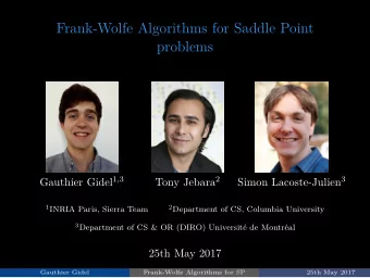
Frank-Wolfe Algorithms for Saddle Point problems Gauthier Gidel 1 Tony Jebara 2 Simon Lacoste-Julien 3 1 INRIA Paris, Sierra Team 2 Department of CS, Columbia University 3 Department of CS & OR (DIRO) Université de Montréal 10th December 2016 Gauthier Gidel Frank-Wolfe Algorithms for SP 10th December 2016

Overview ◮ Frank-Wolfe algorithm (FW) gained in popularity in the last couple of years. ◮ Main advantage: FW only needs LMO. ◮ Extend FW properties to solve saddle point problem. ◮ Straightforward extension but Non trivial analysis. Gauthier Gidel Frank-Wolfe Algorithms for SP 10th December 2016

Saddle point and link with variational inequalities Let L : X × Y → R , where X and Y are convex and compact. Saddle point problem: solve min x ∈X max y ∈Y L ( x , y ) A solution ( x ∗ , y ∗ ) is called a Saddle Point . Gauthier Gidel Frank-Wolfe Algorithms for SP 10th December 2016

Saddle point and link with variational inequalities Let L : X × Y → R , where X and Y are convex and compact. Saddle point problem: solve min x ∈X max y ∈Y L ( x , y ) A solution ( x ∗ , y ∗ ) is called a Saddle Point . ◮ Necessary stationary conditions: � x − x ∗ , ∇ x L ( x ∗ , y ∗ ) � ≥ 0 Gauthier Gidel Frank-Wolfe Algorithms for SP 10th December 2016

Saddle point and link with variational inequalities Let L : X × Y → R , where X and Y are convex and compact. Saddle point problem: solve min x ∈X max y ∈Y L ( x , y ) A solution ( x ∗ , y ∗ ) is called a Saddle Point . ◮ Necessary stationary conditions: � x − x ∗ , ∇ x L ( x ∗ , y ∗ ) � ≥ 0 � y − y ∗ , −∇ y L ( x ∗ , y ∗ ) � ≥ 0 Gauthier Gidel Frank-Wolfe Algorithms for SP 10th December 2016

Saddle point and link with variational inequalities Let L : X × Y → R , where X and Y are convex and compact. Saddle point problem: solve min x ∈X max y ∈Y L ( x , y ) A solution ( x ∗ , y ∗ ) is called a Saddle Point . ◮ Necessary stationary conditions: � x − x ∗ , ∇ x L ( x ∗ , y ∗ ) � ≥ 0 � y − y ∗ , −∇ y L ( x ∗ , y ∗ ) � ≥ 0 ◮ Variational inequality: � z − z ∗ , g ( z ∗ ) � ≥ 0 ∀ z ∈ X × Y where ( x ∗ , y ∗ ) = z ∗ and g ( z ) = ( ∇ x L ( z ) , −∇ y L ( z )) Gauthier Gidel Frank-Wolfe Algorithms for SP 10th December 2016

Saddle point and link with variational inequalities Let L : X × Y → R , where X and Y are convex and compact. Saddle point problem: solve min x ∈X max y ∈Y L ( x , y ) A solution ( x ∗ , y ∗ ) is called a Saddle Point . ◮ Necessary stationary conditions: � x − x ∗ , ∇ x L ( x ∗ , y ∗ ) � ≥ 0 � y − y ∗ , −∇ y L ( x ∗ , y ∗ ) � ≥ 0 ◮ Variational inequality: � z − z ∗ , g ( z ∗ ) � ≥ 0 ∀ z ∈ X × Y where ( x ∗ , y ∗ ) = z ∗ and g ( z ) = ( ∇ x L ( z ) , −∇ y L ( z )) ◮ Sufficient condition : Global solution if L convex-concave . ∀ ( x , y ) ∈ X × Y x ′ �→ L ( x ′ , y ) is convex y ′ �→ L ( x , y ′ ) is concave . and Gauthier Gidel Frank-Wolfe Algorithms for SP 10th December 2016

Motivations: games and robust learning ◮ Zero-sum games with two players: y ∈ ∆( J ) x ⊤ M y x ∈ ∆( I ) max min 1 J. Wen, C. Yu, and R. Greiner. “Robust Learning under Uncertain Test Distributions: Relating Covariate Shift to Model Misspecification.” In: ICML . 2014. Gauthier Gidel Frank-Wolfe Algorithms for SP 10th December 2016

Motivations: games and robust learning ◮ Zero-sum games with two players: y ∈ ∆( J ) x ⊤ M y x ∈ ∆( I ) max min ◮ Generative Adversarial Network (GAN) 1 J. Wen, C. Yu, and R. Greiner. “Robust Learning under Uncertain Test Distributions: Relating Covariate Shift to Model Misspecification.” In: ICML . 2014. Gauthier Gidel Frank-Wolfe Algorithms for SP 10th December 2016

Motivations: games and robust learning ◮ Zero-sum games with two players: y ∈ ∆( J ) x ⊤ M y x ∈ ∆( I ) max min ◮ Generative Adversarial Network (GAN) ◮ Robust learning: 1 We want to learn n 1 � min ℓ ( f θ ( x i ) , y i ) + λ Ω( θ ) n θ ∈ Θ i =1 with an uncertainty regarding the data: n � min θ ∈ Θ max ω i ℓ ( f θ ( x i ) , y i ) + λ Ω( θ ) w ∈ ∆ n i =1 Minimize the worst case → gives robustness 1 J. Wen, C. Yu, and R. Greiner. “Robust Learning under Uncertain Test Distributions: Relating Covariate Shift to Model Misspecification.” In: ICML . 2014. Gauthier Gidel Frank-Wolfe Algorithms for SP 10th December 2016

Problem with Hard projection The structured SVM: n ω ∈ R d λ Ω( ω ) + 1 � min y ∈Y i ( L i ( y ) − � ω, φ i ( y ) � ) max n i =1 � �� � structured hinge loss Gauthier Gidel Frank-Wolfe Algorithms for SP 10th December 2016

Problem with Hard projection The structured SVM: n ω ∈ R d λ Ω( ω ) + 1 � min max y ∈Y i ( L i ( y ) − � ω, φ i ( y ) � ) n i =1 � �� � structured hinge loss Regularization: penalized → constrained. α ∈ ∆( |Y| ) b T α − ω T Mα min max Ω( ω ) ≤ β Gauthier Gidel Frank-Wolfe Algorithms for SP 10th December 2016

Problem with Hard projection The structured SVM: n ω ∈ R d λ Ω( ω ) + 1 � min max y ∈Y i ( L i ( y ) − � ω, φ i ( y ) � ) n i =1 � �� � structured hinge loss Regularization: penalized → constrained. α ∈ ∆( |Y| ) b T α − ω T Mα min max Ω( ω ) ≤ β Gauthier Gidel Frank-Wolfe Algorithms for SP 10th December 2016

Problem with Hard projection The structured SVM: n ω ∈ R d λ Ω( ω ) + 1 � min max y ∈Y i ( L i ( y ) − � ω, φ i ( y ) � ) n i =1 � �� � structured hinge loss Regularization: penalized → constrained. α ∈ ∆( |Y| ) b T α − ω T Mα min max Ω( ω ) ≤ β Gauthier Gidel Frank-Wolfe Algorithms for SP 10th December 2016

Problem with Hard projection The structured SVM: n ω ∈ R d λ Ω( ω ) + 1 � min max y ∈Y i ( L i ( y ) − � ω, φ i ( y ) � ) n i =1 � �� � structured hinge loss Regularization: penalized → constrained. α ∈ ∆( |Y| ) b T α − ω T Mα min max Ω( ω ) ≤ β Hard to project when: Gauthier Gidel Frank-Wolfe Algorithms for SP 10th December 2016

Problem with Hard projection The structured SVM: n ω ∈ R d λ Ω( ω ) + 1 � min max y ∈Y i ( L i ( y ) − � ω, φ i ( y ) � ) n i =1 � �� � structured hinge loss Regularization: penalized → constrained. α ∈ ∆( |Y| ) b T α − ω T Mα min max Ω( ω ) ≤ β Hard to project when: ◮ Structured sparsity norm (group lasso norm). Gauthier Gidel Frank-Wolfe Algorithms for SP 10th December 2016

Problem with Hard projection The structured SVM: n ω ∈ R d λ Ω( ω ) + 1 � min max y ∈Y i ( L i ( y ) − � ω, φ i ( y ) � ) n i =1 � �� � structured hinge loss Regularization: penalized → constrained. α ∈ ∆( |Y| ) b T α − ω T Mα min max Ω( ω ) ≤ β Hard to project when: ◮ Structured sparsity norm (group lasso norm). ◮ The output Y is structured: exponential size. Gauthier Gidel Frank-Wolfe Algorithms for SP 10th December 2016

Standard approaches in literature Simplest algorithm to solve Saddle point problems is the projected gradient algorithm . x ( t +1) = P X ( x ( t ) − η ∇ x L ( x ( t ) , y ( t ) )) y ( t +1) = P Y ( y ( t ) + η ∇ y L ( x ( t ) , y ( t ) )) For non-smooth optimization, T 1 � x ( t ) , y ( t ) � � T →∞ ( x ∗ , y ∗ ) − → T t =1 2 N. He and Z. Harchaoui. “Semi-proximal Mirror-Prox for Nonsmooth Composite Minimization”. In: NIPS . 2015. Gauthier Gidel Frank-Wolfe Algorithms for SP 10th December 2016

Standard approaches in literature Simplest algorithm to solve Saddle point problems is the projected gradient algorithm . x ( t +1) = P X ( x ( t ) − η ∇ x L ( x ( t ) , y ( t ) )) y ( t +1) = P Y ( y ( t ) + η ∇ y L ( x ( t ) , y ( t ) )) For non-smooth optimization, T 1 � x ( t ) , y ( t ) � � T →∞ ( x ∗ , y ∗ ) − → T t =1 Faster algorithm: projected extra-gradient algorithm . 2 N. He and Z. Harchaoui. “Semi-proximal Mirror-Prox for Nonsmooth Composite Minimization”. In: NIPS . 2015. Gauthier Gidel Frank-Wolfe Algorithms for SP 10th December 2016

Standard approaches in literature Simplest algorithm to solve Saddle point problems is the projected gradient algorithm . x ( t +1) = P X ( x ( t ) − η ∇ x L ( x ( t ) , y ( t ) )) y ( t +1) = P Y ( y ( t ) + η ∇ y L ( x ( t ) , y ( t ) )) For non-smooth optimization, T 1 � x ( t ) , y ( t ) � � T →∞ ( x ∗ , y ∗ ) − → T t =1 Faster algorithm: projected extra-gradient algorithm . Can use LMO to compute approximate projections 2 . 2 N. He and Z. Harchaoui. “Semi-proximal Mirror-Prox for Nonsmooth Composite Minimization”. In: NIPS . 2015. Gauthier Gidel Frank-Wolfe Algorithms for SP 10th December 2016

The FW algorithm Algorithm Frank-Wolfe algorithm 1: Let x (0) ∈ X f 2: for t = 0 . . . T do Compute r ( t ) = ∇ f ( x ( t ) ) 3: � s , r ( t ) � Compute s ( t ) ∈ argmin f ( α ) 4: s ∈X � x ( t ) − s ( t ) , r ( t ) � Compute g t := 5: if g t ≤ ǫ then return x ( t ) 6: 2 Let γ = 2+ t (or do line-search) 7: Update x ( t +1) := (1 − γ ) x ( t ) + γ s ( t ) 8: α M 9: end for Gauthier Gidel Frank-Wolfe Algorithms for SP 10th December 2016