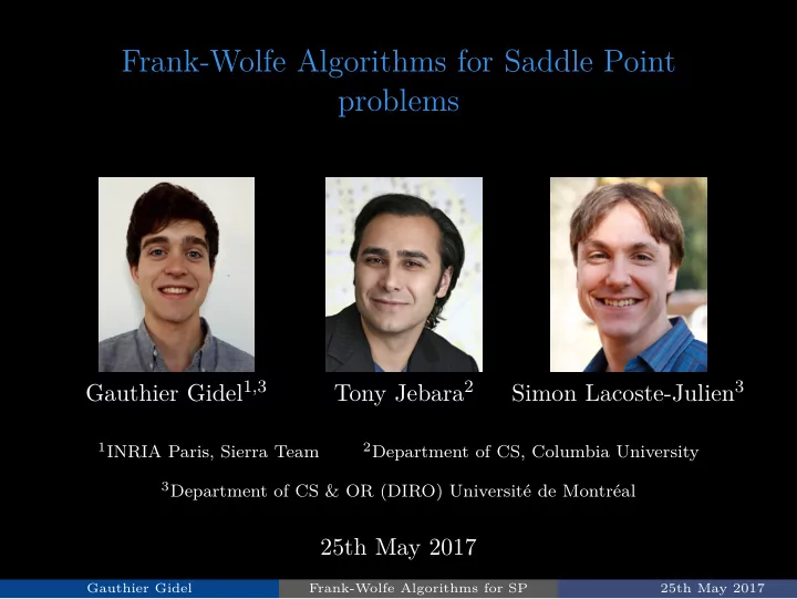
Frank-Wolfe Algorithms for Saddle Point problems Gauthier Gidel 1 , - PowerPoint PPT Presentation
Frank-Wolfe Algorithms for Saddle Point problems Gauthier Gidel 1 , 3 Tony Jebara 2 Simon Lacoste-Julien 3 1 INRIA Paris, Sierra Team 2 Department of CS, Columbia University 3 Department of CS & OR (DIRO) Universit de Montral 25th May 2017
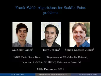
Frank-Wolfe Algorithms for Saddle Point problems Gauthier Gidel 1 , 3 Tony Jebara 2 Simon Lacoste-Julien 3 1 INRIA Paris, Sierra Team 2 Department of CS, Columbia University 3 Department of CS & OR (DIRO) Université de Montréal 25th May 2017 Gauthier Gidel Frank-Wolfe Algorithms for SP 25th May 2017
Overview ◮ Frank-Wolfe algorithm (FW) gained in popularity in the last couple of years. ◮ Main advantage: FW only needs LMO. ◮ Extend FW properties to solve saddle point problem 1 . ◮ Straightforward extension but Non trivial analysis. 1 Gauthier Gidel, Tony Jebara, and Simon Lacoste-Julien. “Frank-Wolfe Algorithms for Saddle Point Problems”. In: AISTATS . 2017. Gauthier Gidel Frank-Wolfe Algorithms for SP 25th May 2017
Overview ◮ Frank-Wolfe algorithm (FW) gained in popularity in the last couple of years. ◮ Main advantage: FW only needs LMO. ◮ Extend FW properties to solve saddle point problem 1 . ◮ Straightforward extension but Non trivial analysis. Question for the audience: Call for application 1 Gauthier Gidel, Tony Jebara, and Simon Lacoste-Julien. “Frank-Wolfe Algorithms for Saddle Point Problems”. In: AISTATS . 2017. Gauthier Gidel Frank-Wolfe Algorithms for SP 25th May 2017
Saddle point and link with variational inequalities Let L : X × Y → R , where X and Y are convex and compact. Saddle point problem: solve min x ∈X max y ∈Y L ( x , y ) A solution ( x ∗ , y ∗ ) is called a Saddle Point . Gauthier Gidel Frank-Wolfe Algorithms for SP 25th May 2017
Saddle point and link with variational inequalities Let L : X × Y → R , where X and Y are convex and compact. Saddle point problem: solve min x ∈X max y ∈Y L ( x , y ) A solution ( x ∗ , y ∗ ) is called a Saddle Point . ◮ Necessary stationary conditions: � x − x ∗ , ∇ x L ( x ∗ , y ∗ ) � ≥ 0 Gauthier Gidel Frank-Wolfe Algorithms for SP 25th May 2017
Saddle point and link with variational inequalities Let L : X × Y → R , where X and Y are convex and compact. Saddle point problem: solve min x ∈X max y ∈Y L ( x , y ) A solution ( x ∗ , y ∗ ) is called a Saddle Point . ◮ Necessary stationary conditions: � x − x ∗ , ∇ x L ( x ∗ , y ∗ ) � ≥ 0 � y − y ∗ , −∇ y L ( x ∗ , y ∗ ) � ≥ 0 Gauthier Gidel Frank-Wolfe Algorithms for SP 25th May 2017
Saddle point and link with variational inequalities Let L : X × Y → R , where X and Y are convex and compact. Saddle point problem: solve min x ∈X max y ∈Y L ( x , y ) A solution ( x ∗ , y ∗ ) is called a Saddle Point . ◮ Necessary stationary conditions: � x − x ∗ , ∇ x L ( x ∗ , y ∗ ) � ≥ 0 � y − y ∗ , −∇ y L ( x ∗ , y ∗ ) � ≥ 0 ◮ Variational inequality: � z − z ∗ , g ( z ∗ ) � ≥ 0 ∀ z ∈ X × Y where ( x ∗ , y ∗ ) = z ∗ and g ( z ) = ( ∇ x L ( z ) , −∇ y L ( z )) Gauthier Gidel Frank-Wolfe Algorithms for SP 25th May 2017
Saddle point and link with variational inequalities Let L : X × Y → R , where X and Y are convex and compact. Saddle point problem: solve min x ∈X max y ∈Y L ( x , y ) A solution ( x ∗ , y ∗ ) is called a Saddle Point . ◮ Necessary stationary conditions: � x − x ∗ , ∇ x L ( x ∗ , y ∗ ) � ≥ 0 � y − y ∗ , −∇ y L ( x ∗ , y ∗ ) � ≥ 0 ◮ Variational inequality: � z − z ∗ , g ( z ∗ ) � ≥ 0 ∀ z ∈ X × Y where ( x ∗ , y ∗ ) = z ∗ and g ( z ) = ( ∇ x L ( z ) , −∇ y L ( z )) ◮ Sufficient condition : Global solution if L convex-concave . ∀ ( x , y ) ∈ X × Y x ′ �→ L ( x ′ , y ) is convex y ′ �→ L ( x , y ′ ) is concave . and Gauthier Gidel Frank-Wolfe Algorithms for SP 25th May 2017
Motivations: games and robust learning ◮ Zero-sum games with two players: y ∈ ∆( J ) x ⊤ M y x ∈ ∆( I ) max min 2 J. Wen, C. Yu, and R. Greiner. “Robust Learning under Uncertain Test Distributions: Relating Covariate Shift to Model Misspecification.” In: ICML . 2014. Gauthier Gidel Frank-Wolfe Algorithms for SP 25th May 2017
Motivations: games and robust learning ◮ Zero-sum games with two players: y ∈ ∆( J ) x ⊤ M y x ∈ ∆( I ) max min ◮ Robust learning: 2 We want to learn n 1 � min ℓ ( f θ ( x i ) , y i ) + λ Ω( θ ) n θ ∈ Θ i =1 with an uncertainty regarding the data: n � min θ ∈ Θ max ω i ℓ ( f θ ( x i ) , y i ) + λ Ω( θ ) w ∈ ∆ n i =1 Minimize the worst case → gives robustness 2 J. Wen, C. Yu, and R. Greiner. “Robust Learning under Uncertain Test Distributions: Relating Covariate Shift to Model Misspecification.” In: ICML . 2014. Gauthier Gidel Frank-Wolfe Algorithms for SP 25th May 2017
Problem with Hard projection The structured SVM: n ω ∈ R d λ Ω( ω ) + 1 � min y ∈Y i ( L i ( y ) − � ω, φ i ( y ) � ) max n i =1 � �� � structured empirical loss Gauthier Gidel Frank-Wolfe Algorithms for SP 25th May 2017
Problem with Hard projection The structured SVM: n ω ∈ R d λ Ω( ω ) + 1 � min max y ∈Y i ( L i ( y ) − � ω, φ i ( y ) � ) n i =1 � �� � structured empirical loss Regularization: penalized → constrained. α ∈ ∆( |Y| ) b T α − ω T Mα min max Ω( ω ) ≤ β Gauthier Gidel Frank-Wolfe Algorithms for SP 25th May 2017
Problem with Hard projection The structured SVM: n ω ∈ R d λ Ω( ω ) + 1 � min max y ∈Y i ( L i ( y ) − � ω, φ i ( y ) � ) n i =1 � �� � structured empirical loss Regularization: penalized → constrained. α ∈ ∆( |Y| ) b T α − ω T Mα min max Ω( ω ) ≤ β Gauthier Gidel Frank-Wolfe Algorithms for SP 25th May 2017
Problem with Hard projection The structured SVM: n ω ∈ R d λ Ω( ω ) + 1 � min max y ∈Y i ( L i ( y ) − � ω, φ i ( y ) � ) n i =1 � �� � structured empirical loss Regularization: penalized → constrained. α ∈ ∆( |Y| ) b T α − ω T Mα min max Ω( ω ) ≤ β Gauthier Gidel Frank-Wolfe Algorithms for SP 25th May 2017
Problem with Hard projection The structured SVM: n ω ∈ R d λ Ω( ω ) + 1 � min max y ∈Y i ( L i ( y ) − � ω, φ i ( y ) � ) n i =1 � �� � structured empirical loss Regularization: penalized → constrained. α ∈ ∆( |Y| ) b T α − ω T Mα min max Ω( ω ) ≤ β Difficult to project when: Gauthier Gidel Frank-Wolfe Algorithms for SP 25th May 2017
Problem with Hard projection The structured SVM: n ω ∈ R d λ Ω( ω ) + 1 � min max y ∈Y i ( L i ( y ) − � ω, φ i ( y ) � ) n i =1 � �� � structured empirical loss Regularization: penalized → constrained. α ∈ ∆( |Y| ) b T α − ω T Mα min max Ω( ω ) ≤ β Difficult to project when: ◮ Structured sparsity norm (group lasso norm). Gauthier Gidel Frank-Wolfe Algorithms for SP 25th May 2017
Problem with Hard projection The structured SVM: n ω ∈ R d λ Ω( ω ) + 1 � min max y ∈Y i ( L i ( y ) − � ω, φ i ( y ) � ) n i =1 � �� � structured empirical loss Regularization: penalized → constrained. α ∈ ∆( |Y| ) b T α − ω T Mα min max Ω( ω ) ≤ β Difficult to project when: ◮ Structured sparsity norm (group lasso norm). ◮ The output Y is structured: exponential size. Gauthier Gidel Frank-Wolfe Algorithms for SP 25th May 2017
Standard approaches in literature ◮ Projected gradient algorithm. x ( t +1) = P X ( x ( t ) − η ∇ x L ( x ( t ) , y ( t ) )) y ( t +1) = P Y ( y ( t ) + η ∇ y L ( x ( t ) , y ( t ) )) 3 GM Korpelevich. “The extragradient method for finding saddle points and other problems”. In: Matecon (1976). Gauthier Gidel Frank-Wolfe Algorithms for SP 25th May 2017
Standard approaches in literature ◮ Projected gradient algorithm. x ( t +1) = P X ( x ( t ) − η ∇ x L ( x ( t ) , y ( t ) )) y ( t +1) = P Y ( y ( t ) + η ∇ y L ( x ( t ) , y ( t ) )) ◮ Projected extra-gradient 3 . x ( t +1) = P X ( x ( t ) − η ∇ x L ( x ( t ) , y ( t ) )) ¯ y ( t +1) = P Y ( y ( t ) + η ∇ y L ( x ( t ) , y ( t ) )) ¯ Intuition: lookahead move: look at what your opponent would do before deciding your move. x ( t +1) = P X ( x ( t ) − η ∇ x L (¯ x ( t +1) , ¯ y ( t +1) )) y ( t +1) = P Y ( y ( t ) + η ∇ y L (¯ x ( t +1) , ¯ y ( t +1) )) Prevents oscillations for non strongly convex objective. 3 GM Korpelevich. “The extragradient method for finding saddle points and other problems”. In: Matecon (1976). Gauthier Gidel Frank-Wolfe Algorithms for SP 25th May 2017
Standard approaches in literature ◮ Gradient method works for non-smooth optimization, but T 1 � x ( t ) , y ( t ) � � T →∞ ( x ∗ , y ∗ ) − → T t =1 4 N. He and Z. Harchaoui. “Semi-proximal Mirror-Prox for Nonsmooth Composite Minimization”. In: NIPS . 2015. Gauthier Gidel Frank-Wolfe Algorithms for SP 25th May 2017
Standard approaches in literature ◮ Gradient method works for non-smooth optimization, but T 1 � x ( t ) , y ( t ) � � T →∞ ( x ∗ , y ∗ ) − → T t =1 ◮ Extragradient method works for smooth optimization, ( x ( t ) , y ( t ) ) → ( x ∗ , y ∗ ) 4 N. He and Z. Harchaoui. “Semi-proximal Mirror-Prox for Nonsmooth Composite Minimization”. In: NIPS . 2015. Gauthier Gidel Frank-Wolfe Algorithms for SP 25th May 2017
Recommend
More recommend
Explore More Topics
Stay informed with curated content and fresh updates.
