FOURIER ANALYSIS OF NUMERICAL INTEGRATION IN MONTE CARLO RENDERING - PowerPoint PPT Presentation
FOURIER ANALYSIS OF NUMERICAL INTEGRATION IN MONTE CARLO RENDERING Kartic Subr Gurprit Singh Wojciech Jarosz Heriot Watt University, Edinburgh Dartmouth College Dartmouth College Motivation for
FOURIER ANALYSIS OF NUMERICAL INTEGRATION IN MONTE CARLO RENDERING Kartic Subr Gurprit Singh Wojciech Jarosz Heriot Watt University, Edinburgh Dartmouth College Dartmouth College
Motivation for analysis • assess, compare existing methods for Monte Carlo rendering • provide insight, inspire improvement
[Subr et al 2014]
Error vs cost plots of rendering methods method 1 method 2 [Subr et al 2014] method 3 method 4
Error vs cost plots of rendering methods method 4 is best method 4 is worst method 1 method 2 [Subr et al 2014] method 3 method 4
Error vs cost plots of rendering methods method 4 is worst method 4 is best method 1 method 2 [Subr et al 2014] method 3 method 4
Course structure 30m 20m Preliminaries Sampling 30m Formal treatment
Rendering = geometry + radiometry radiometrically accurate simulation geometry/projection is important for photorealism for pin-hole model known since 400BC OpenGL Raytracing [Stachowiak 2010] [Whitted 1980] camera obscura [photo credit: videomaker.com June 2015]
Rendering = geometry + radiometry radiometrically accurate simulation geometry/projection is important for photorealism for pin-hole model known since 400BC OpenGL Raytracing [Stachowiak 2010] [Whitted 1980] [photo credit: videomaker.com June 2015]
Radiometric fidelity improves photorealism manually painted computer generated photograph Pedro Campos Colourbox.com
Simulating the physics of light is challenging defocus exposure time lenses light, media materials
Light transport virtual virtual camera light emitter virtual scene: geometry + materials estimate incident Image ? radiance at all pixels on the virtual sensor exitant radiance W m 2 Sr 12
Each reflection is modeled by an integration radiance: 13
Each reflection is modeled by an integration radiance: 14
Each reflection is modeled by an integration radiance: 15
Recursive integrals virtual virtual camera light emitter Image ? 16
Recursive integrals virtual virtual camera light emitter Image ? 17
Light transport: recursive integral equation radiance emitted radiance integral operator The Rendering equation [Kajiya 86] Light Transport Operators [Arvo 94] 18
L is a sum of high-dimensional integrals radiance integral operator emitted radiance One bounce Three bounces 19
Reconstruction and integration in rendering
Reconstruction: estimate image samples reconstruct on (low-res) pixel grid ground truth (high-res) image Y Y X X
Naïve method: sample image at grid locations reconstruct on (low-res) pixel grid ground truth (high-res) image Y Y copy sampling X X
Naïve method: when sampling is increased reconstruct on (low-res) pixel grid ground truth (high-res) image aliasing Y Y X X
Antialiasing: assuming `square’ pixels Y Y average multi-sampling X X
Antialiasing is costly due to multi-sampling Y Y X X
Antialiasing using general reconstruction filter Y Y weighted multi-sampling average X X
Rendering: Reconstructing integrals multi-sampling for reconstruction deterministic
Rendering: Reconstructing integrals path 1 path 2 multi-path sampling multi-sampling for integration for reconstruction estimate per sampled pixel path 3 estimate (probabilistic for Monte Carlo)
Function-space view: Sampling in path space each sample represents a path light and has an associated radiance value light paths camera n-dimensional path space 29
Sample locations shown in path-pixel space n-dimensional path space pixels on sensor 30
Rendering = integration + reconstruction n-dimensional path space pixel value (radiance) path-space integration (projection) reconstruction using integrated radiance pixels on sensor pixels on sensor 31
Frequency analysis of lightfields in rendering reconstruction filter local variation of integrand n-dimensional path space path-space integration pixel value (radiance) (projection) integrated radiance local variation/ anisotropy? use in regression/reconstruction [Ramamoorthi et al. 04] pixels on sensor pixels on sensor [Durand et al. 05] [Soler et al. 2009] [Overbeck et al. 2009] [Egan et al. 2009, 2011] [Ramamoorthi et al. 2012]
Freq. analysis of MC sampling: This course! Assessing MSE, bias, variance and convergence of Monte Carlo estimators as a function of the n-dimensional path space Fourier spectrum of the sampling function. local variation/ anisotropy? pixels on sensor [Durand 2011] [Ramamoorthi et al. 12] [Subr and Kautz 2013] [Pilleboue et al. 2015]
Freq. analysis of MC sampling: This course! Assessing MSE, bias, variance and convergence of Monte Carlo estimators as a function of the n-dimensional path space Fourier spectrum of the sampling function. [Durand 2011] [Ramamoorthi et al. 12] [Subr and Kautz 2013] [Pilleboue et al. 2015]
Freq. analysis of MC sampling: This course! Assessing MSE, bias, variance and convergence of Monte Carlo estimators as a function of the n-dimensional path space Fourier spectrum of the sampling function. local variation/ anisotropy? [Durand 2011] [Ramamoorthi et al. 12] [Subr and Kautz 2013] [Pilleboue et al. 2015]
Rendering = integration + reconstruction Shiny ball in motion Shiny ball, out of focus … … image location multi-dim integral Integrand: radiance (W m -2 Sr -1 ) Domain: shutter time x aperture area x 1 st bounce x 2 nd bounce … 38
Th The prob oble lem in in 1D 0 39
the sampling funct ction integrand sampled integrand sampling function multiply 40
sampling funct ction deci cides integration qua quality ty integrand sampled function sampling function multiply 41
st strategies to improve est stimators 1. modify weights 2. modify locations eg. quadrature rules, importance sampling, jittered sampling, etc. 42
in insig ight t in into im impac act: t: Fourier ier domain ain 1. modify weights 2. modify locations analyse sampling function in Fourier domain 43
Fourier analysis: origin and intuition • Eigenfunction of the differential operator scaling • Turns differential equations into algebraic equations
Fourier analysis: origin and intuition • Eigenfunction of the differential operator scaling • Turns differential equations into algebraic equations • if projection
The Fourier domain Image credit: Wikipedia
The continuous Fourier transform primal Fourier (space, time, etc.) domain domain
The Fourier transform: `frequency’ domain frequency frequency domain projection onto sin and cos
A single sample: phase amplitude = 1 frequency
Fourier series: replace integral with sum approximating a square wave using 4 sinusoids
Fourier spectrum of the sampling function amplitude (sampling spectrum) sampling function frequency phase (sampling spectrum) 51
sa sampling g fu function = = su sum of f Dirac deltas + + +
In In th the e Fourier ier domain ain … Fourier transform Dirac delta Frequency Imaginary amplitude phase Real primal Fourier Complex plane
Re Review: in the Fourier domain … Fourier transform Dirac delta Frequency Imaginary Imaginary Real Real primal Fourier Complex plane Complex plane
am amplitu litude e spec ectr trum is is not t fla lat Fourier transform = = + + + + + + primal Fourier
sa sample contributions s at a gi given fr frequency 1 2 3 4 5 At a given frequency sampling function Imaginary 3 5 Real 1 4 2 Complex plane
th the e sam amplin ling spec ectr trum at t a a giv iven en freq equen ency sampling spectrum Complex plane given frequency 3 5 centroid 1 4 2
th the e sam amplin ling spec ectr trum at t a a giv iven en freq equen ency sampling spectrum realizations centroid variance expected centroid given frequency
ex expected sampling spectrum and va variance expected amplitude of sampling spectrum variance of sampling spectrum DC frequency
Ab Abstracting ng sa sampl pling ng strategy gy usi using ng spe spectra 1. modify weights 2. modify locations sampling function in the Fourier domain amplitude (sampling spectrum) eg. quadrature rules a. Distribution eg. importance sampling) frequency phase (sampling spectrum) 60
Recommend
More recommend
Explore More Topics
Stay informed with curated content and fresh updates.

