Formal Verifjcation Lecture 7: Introduction to Binary Decision - PowerPoint PPT Presentation
Formal Verifjcation Lecture 7: Introduction to Binary Decision Diagrams (BDDs) Jacques Fleuriot jdf@inf.ac.uk Diagrams from Huth & Ryan, 2nd Ed. Recap Previously: CTL and LTL Model Checking algorithms Tiis time: Binary
Formal Verifjcation Lecture 7: Introduction to Binary Decision Diagrams (BDDs) Jacques Fleuriot jdf@inf.ac.uk Diagrams from Huth & Ryan, 2nd Ed.
Recap ▶ Previously: ▶ CTL and LTL Model Checking algorithms ▶ Tiis time: ▶ Binary Decision Diagrams ▶ Reduced Binary Decision Diagrams ▶ Reduced Ordered Binary Decision Diagrams
Model Checling needs Very Large Sets ###################################################################### petabytes to explicitly store the set of all reachable approx If each state is represented using 96 bits, it would need at least ###################################################################### reachable states: 2.10443e+14 (2^47.5804) out of 2.63684e+27 (2^91.0909) system diameter: 70 NuSMV > print_reachable_states According to NuSMV: guidance , which is a model of part of the Shutule’s autopilot. Example: Tie NuSMV 2.6 distribution contains an example For realistic models, the size of S can be enormous. checking algorithm translates CTL formulas into sets of states: states. Given a model M = ⟨ S , S 0 , → , L ⟩ and a formula φ , the CTL model � φ � ⊆ S
Model Checling needs Very Large Sets checking algorithm translates CTL formulas into sets of states: For realistic models, the size of S can be enormous. Example: Tie NuSMV 2.6 distribution contains an example guidance , which is a model of part of the Shutule’s autopilot. According to NuSMV: NuSMV > print_reachable_states ###################################################################### system diameter: 70 reachable states: 2.10443e+14 (2^47.5804) out of 2.63684e+27 (2^91.0909) ###################################################################### If each state is represented using 96 bits, it would need at least states. Given a model M = ⟨ S , S 0 , → , L ⟩ and a formula φ , the CTL model � φ � ⊆ S approx 2 . 52 petabytes to explicitly store the set of all reachable
Representing states as Boolean functions Idea: represent sets of states as boolean functions. Tie set of all states could be represented as: 1. a data structure with nodes; or 2. the boolean function: f w How to represent boolean functions? 1. Represent each state as a binary string in { 0 , 1 } k 2. Represent a set of states as a function f : { 0 , 1 } k → { 0 , 1 } f ( w ) = 1 if the state represented by w is in the set f ( w ) = 0 if the state represented by w is not in the set ⇒ representation of sets by their ciaracteristic functions
Representing states as Boolean functions Idea: represent sets of states as boolean functions. Tie set of all states could be represented as: 2. the boolean function: How to represent boolean functions? 1. Represent each state as a binary string in { 0 , 1 } k 2. Represent a set of states as a function f : { 0 , 1 } k → { 0 , 1 } f ( w ) = 1 if the state represented by w is in the set f ( w ) = 0 if the state represented by w is not in the set ⇒ representation of sets by their ciaracteristic functions 1. a data structure with 2 . 63684 × 10 27 nodes; or f ( w ) = 1
Representations of Boolean Functions Reduced OBDDs easy hard hard Truth Tables never hard hard hard hard hard ofuen hard easy easy medium medium easy Space complexity of representations and time complexities of operations on those representations. Note: With a truth table representation, while operations are conceptually easy, especially when table rows are always listed in some standard order, the time complexities are hard, as table sizes and hence operation time complexities are easy sometimes From H&R, Figure 6.1 hard test for Operations Representation compact? satisf’y validity Prop. Formulas ofuen Formulas in CNF hard easy easy easy Formulas in DNF sometimes easy hard hard easy hard always exponential in the number of input variables. ∧ ∨ ¬
Binary decision trees y 1. Start at root To compute value: Note on notation: � � y � � 4. Function value is value at terminal node reached x � � Tree for the boolean function f ( x , y ) · = ¬ x ∧ ¬ y ���� ���� ❀ ❀ ❀ ❀ ❀ ❀ ❀ ❀ ���� ���� ���� ���� ✳ ✳ ✳ ✳ ✳ ✳ ✳ ✳ ✳ ✳ ✳ ✳ 1 0 0 0 ▶ 0, 1 for ⊥ (False), ⊤ (True) ▶ Ofuen also have: + , · , ¯ for ∨ , ∧ , ¬ 2. Take dashed line if value of var at current node is 0 3. Take solid line if value of var at current node is 1
Binary decision diagram Similar to Binary Decision Trees, except that nodes can have multiple in-edges. A binary decision diagram (BDD) is a fjnite DAG (Directed Acyclic Graph) with: We will use BDDs with two extra properties: 1. Reduced – eliminate redundancy 2. Ordered – canonical ordering of the boolean variables ▶ a unique initial node; ▶ all non-terminals labelled with a boolean variable; ▶ all terminals labelled with 0 or 1 ; ▶ all edges are labelled 0 (dashed) or 1 (solid); ▶ each non-terminal has exactly: one out-edge labelled 0 , and one out-edge labelled 1 .
Reducing BDDs I � � x redundant � � remove y � � y remove duplicate terminals x � � � y y � � y x � � � ���� ���� ���� ���� ❁ ❁ ❁ ❁ ❁ ❁ ❁ ❁ ❁ ❁ ❁ ❁ ❁ ❁ ❁ ❁ − → ���� ���� ���� ���� ���� ���� ���� ���� ● ✳ ✳ ● ● ✳ ✳ ● ✳ ✳ ● ✳ ✳ ● ● ✳ ✳ ● ✳ ✳ ● ● � � 1 0 0 0 1 0 ���� ���� ✫ ✫ ✫ ✫ test − → ✫ ✫ ✫ ���� ���� ✫ ✫ ● ● ✫ ● ● ✫ ● ✫ ● ● ✫ ● � � ✫ ● ● 1 0
Reducing BDDs II � � y � � � y � y � � � y x Removing duplicate non-terminals: y � � y � z � � x x � � x z � � � � ���� ���� ���� ���� − → ❅ ✽ ❅ ✽ ❅ ✽ ❅ ✽ ❅ ❅ ✽ ❅ ✽ ❅ ✽ ❅ ���� ���� ���� ���� ���� ���� ���� ���� ✴ ✴ ✴ ✴ ✴ ✴ ✴ ✴ ✴ ✴ ✴ ✴ ✴ ✴ ✴ ✴ ✴ ✴ � � ���� ���� ���� ���� ���� ���� ���� ���� ���� ���� ���� ���� ❙ ❙ � ❦❦❦❦❦❦❦❦❦❦❦❦❦❦❦❦❦❦❦❦ ❑ � ❧❧❧❧❧❧❧❧❧❧❧❧❧❧❧❧❧❧ ● ❙ ❑ ❙ ✵ ● ❙ ❑ ● ❙ ❑ ✵ ❙ ● ❙ ❑ ✵ ❙ ● ❙ ❑ ❙ ❑ ✵ ● ❙ ❙ ❑ ● ❙ ❑ ✵ ● ❙ ❑ ❙ ✵ ● ❙ ❑ ❙ ● ❑ ❙ ❙ 0 1 0 1
Reducing BDDs III z � y � � y � Removing redundant test: � x � x � � y � � � � y z � � x ���� ���� ���� ���� − → ✽ ✽ ✽ ✽ ✽ ✽ ✽ ✽ ✽ ✽ ✽ ✽ ✽ ✽ ���� ���� ���� ���� ���� ���� ✴ ✴ ✴ ✴ ✴ ✴ ✴ ✴ ✴ ✴ ✴ ✴ � � ���� ���� ���� ���� ���� ���� ���� ���� � ❧❧❧❧❧❧❧❧❧❧❧❧❧❧❧❧❧❧ ● ● � ♠♠♠♠♠♠♠♠♠♠♠♠♠♠♠♠♠ ● ● ● ● ● ● ● ● ● ● ● ● ● ● ● ● ● ● 0 1 0 1
Reduction Operations 2. Removal of redundant tests. If both outgoing edges of a node n point to the same node m , then remove node n , sending all its incoming edges to m . 3. Removal of duplicate non-terminals. If two distinct nodes n and m in the BDD are the roots of structurally identical subBDDs, then eliminate one of them and redirect all its incoming edges to the other one. All of these operations preserve the BDD-ness of the DAG. A BDD is reduced if it has been simplifjed as much as possible using these reduction operations. 1. Removal of duplicate terminals. If a BDD contains more than one terminal 0 -node, then redirect all edges which point to such a 0 -node to just one of them. Do the same with terminal nodes labelled 1 .
Generality of BDDs � � y � � x � z � y � x x � � x � � y � A variable might occur more than once on a path � � Ordering of variables on paths is not fjxed � x � � y � � � z ���� ���� ���� ���� ✵ ✵ ✵ ✵ ✵ ✵ ✵ ✵ ✵ ✵ ✵ ✵ ✵ ✵ ���� ���� ���� ���� ���� ���� ���� ���� ✴ ✴ ✵ ✴ ✴ ✵ ✴ ✴ ✵ ✴ ✴ ✵ ✴ ✴ ✵ ✴ ✴ ✵ ✴ ✴ ✵ ✵ ���� ���� ���� ���� ���� ���� ���� ���� ���� ���� ✵ ✵ ▲ ▲ ▲ ▲ ✶ ✵ ▲ ▲ ▲ � ✍✍✍✍✍✍ ▲ ✵ ✶ � ✌✌✌✌✌✌ ▲ ▲ ▲ ✶ ▲ ✵ ▲ ▲ ✶ ✵ ▲ ▲ ▲ ▲ ✶ ✵ ▲ ▲ ▲ ✶ ▲ ✵ ▲ ▲ ▲ ▲ 0 1 0 1
Recommend
More recommend
Explore More Topics
Stay informed with curated content and fresh updates.
