Fixed-point Characterization of Compositionality Properties of - PowerPoint PPT Presentation

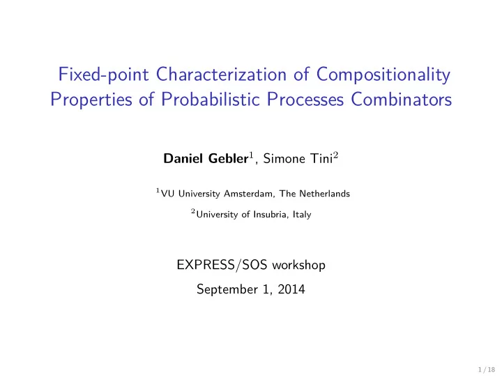
Fixed-point Characterization of Compositionality Properties of Probabilistic Processes Combinators EXPRESS/SOS workshop September 1, 2014 1 / 18 Daniel Gebler 1 , Simone Tini 2 1 VU University Amsterdam, The Netherlands 2 University of Insubria, Italy

d t n t n Motivation: Metric compositionality in a nutshell t n given any operator specification, what is its modulus of continuity? specified operator admits this modulus of continuity? given any modulus of continuity, what are the syntactical properties s.t. a which process algebra operators are continuous? This talk: Metric compositionality = congruence of kernel relation + modulus of continuity f . for some modulus of continuity n f t n f t n d f t t d t is continuous wrt. behavioral distance d if: An operation f n 2 / 18 An operation f ∈ Σ is congruent wrt. behavioral relation ∼ if: t 1 ∼ t ′ t n ∼ t ′ . . . 1 f ( t 1 , . . . , t n ) ∼ f ( t ′ 1 , . . . , t ′ n )

Motivation: Metric compositionality in a nutshell Metric compositionality = congruence of kernel relation + modulus of continuity given any operator specification, what is its modulus of continuity? specified operator admits this modulus of continuity? given any modulus of continuity, what are the syntactical properties s.t. a which process algebra operators are continuous? This talk: 2 / 18 n An operation f ∈ Σ is congruent wrt. behavioral relation ∼ if: t 1 ∼ t ′ t n ∼ t ′ . . . 1 f ( t 1 , . . . , t n ) ∼ f ( t ′ 1 , . . . , t ′ n ) An operation f ∈ Σ is continuous wrt. behavioral distance d if: d ( t 1 , t ′ d ( t n , t ′ 1 ) ≤ ϵ 1 . . . n ) ≤ ϵ n d ( f ( t 1 , . . . , t n ) , f ( t ′ 1 , . . . , t ′ n )) ≤ ω f ( ϵ 1 , . . . , ϵ n ) for some modulus of continuity ω f .

Motivation: Metric compositionality in a nutshell Metric compositionality = congruence of kernel relation + modulus of continuity given any operator specification, what is its modulus of continuity? specified operator admits this modulus of continuity? given any modulus of continuity, what are the syntactical properties s.t. a which process algebra operators are continuous? This talk: 2 / 18 n An operation f ∈ Σ is congruent wrt. behavioral relation ∼ if: t 1 ∼ t ′ t n ∼ t ′ . . . 1 f ( t 1 , . . . , t n ) ∼ f ( t ′ 1 , . . . , t ′ n ) An operation f ∈ Σ is continuous wrt. behavioral distance d if: d ( t 1 , t ′ d ( t n , t ′ 1 ) ≤ ϵ 1 . . . n ) ≤ ϵ n d ( f ( t 1 , . . . , t n ) , f ( t ′ 1 , . . . , t ′ n )) ≤ ω f ( ϵ 1 , . . . , ϵ n ) for some modulus of continuity ω f .

Motivation: Metric compositionality in a nutshell Metric compositionality = congruence of kernel relation + modulus of continuity given any operator specification, what is its modulus of continuity? specified operator admits this modulus of continuity? given any modulus of continuity, what are the syntactical properties s.t. a which process algebra operators are continuous? This talk: 2 / 18 n An operation f ∈ Σ is congruent wrt. behavioral relation ∼ if: t 1 ∼ t ′ t n ∼ t ′ . . . 1 f ( t 1 , . . . , t n ) ∼ f ( t ′ 1 , . . . , t ′ n ) An operation f ∈ Σ is continuous wrt. behavioral distance d if: d ( t 1 , t ′ d ( t n , t ′ 1 ) ≤ ϵ 1 . . . n ) ≤ ϵ n d ( f ( t 1 , . . . , t n ) , f ( t ′ 1 , . . . , t ′ n )) ≤ ω f ( ϵ 1 , . . . , ϵ n ) for some modulus of continuity ω f .

Probabilistic Transition Systems a (countable) set of states S a (countable) set of actions A 3 / 18 A probabilistic transition system ( S , A , − → ) consists of a transition relation − → ⊆ S × A × ∆( S ) with ∆( S ) the set of probability distributions over S .

Perturbation of probabilities and bisimulation equivalence . c . . . q . . . . . Implementation b . a . . . b . c . . . . . . p . . . . . . Specification 4 / 18 . a . . d p q . ̸∼ ◦ ◦ 0 . 6 0 . 4 0 . 6 − ϵ 0 . 4 + ϵ p 2 p 3 q 2 q 3 1 . 0 1 . 0 1 . 0 1 . 0 ◦ ◦ ◦ ◦

Perturbation of probabilities and bisimulation equivalence . c . . . q . . . . . Implementation b . a . . . b . c . . . . . . p . . . . . . Specification 4 / 18 . a . . d p q . ̸∼ ◦ ◦ 0 . 6 0 . 4 0 . 6 − ϵ 0 . 4 + ϵ p 2 p 3 q 2 q 3 1 . 0 1 . 0 1 . 0 1 . 0 ◦ ◦ ◦ ◦

Perturbation of probabilities and bisimulation equivalence . . . . q . . . . . Implementation . . a . . . b . c . . c . b . p . . . . . . . Specification . 4 / 18 a . . . d ( p , q ) = ϵ ◦ ◦ 0 . 6 0 . 4 0 . 6 − ϵ 0 . 4 + ϵ p 2 p 3 q 2 q 3 1 . 0 1 . 0 1 . 0 1 . 0 ◦ ◦ ◦ ◦

Bisimulation metrics between PTS . . . . a . a . . . . . 5 / 18 A pseudometric d : S × S → [0 , 1] is a bisimulation metric if d ( s 1 , s 2 ) ≤ ϵ s 1 s 2 ∀ ∃ π 1 K ( d )( π 1 , π 2 ) ≤ ϵ π 2 with K ( d ): ∆( S ) × ∆( S ) → [0 , 1] lifts state metric d to distributions.

Bisimulation metrics between PTS . . . . a . a . . . . . 5 / 18 A pseudometric d : S × S → [0 , 1] is a bisimulation metric if d ( s 1 , s 2 ) ≤ ϵ s 1 s 2 ∀ ∃ π 1 K ( d )( π 1 , π 2 ) ≤ ϵ π 2 with K ( d ): ∆( S ) × ∆( S ) → [0 , 1] lifts state metric d to distributions.

Bisimulation metric by example . . . a . . . . b . . . . . . q . . . . . . . . q d p d p q . . . . d . c . . 6 / 18 . . . . . a . . . . b . . . c . p . . d . . ◦ ◦ 1/3 1/3 2/3 2/3 • • p 2 q 2 ◦ ◦ 0 . 4 + ϵ 0 . 6 − ϵ 0 . 6 0 . 4 p ′ q ′ d ( p 3 , q 3 ) = 0 p 3 q 3 3 3 d ( p ′ 3 , q ′ 3 ) = 0 1 . 0 1 . 0 1 . 0 1 . 0 ◦ ◦ d ( p 3 , q ′ ◦ ◦ 3 ) = 1 d ( p ′ 3 , q 3 ) = 1

Bisimulation metric by example . . a . . . . . . . . . . q . . b . . . . . . . d p q . . . d . c . . . . d . p . . . . . . . . a . . . 6 / 18 . b . . c . ◦ ◦ 1/3 1/3 2/3 2/3 • d ( p 2 , q 2 ) = ϵ • p 2 q 2 ◦ ◦ 0 . 4 + ϵ 0 . 6 − ϵ 0 . 6 0 . 4 p ′ q ′ d ( p 3 , q 3 ) = 0 p 3 q 3 3 3 d ( p ′ 3 , q ′ 3 ) = 0 1 . 0 1 . 0 1 . 0 1 . 0 ◦ ◦ d ( p 3 , q ′ ◦ ◦ 3 ) = 1 d ( p ′ 3 , q 3 ) = 1

Bisimulation metric by example . . q . . . . . . . . . . a . . . . . . . . . . . b d . c . . . . . d . p . . . . . . . . . . a . 6 / 18 . c . b . . d ( p , q ) = 1 / 3 · ϵ ◦ ◦ 1/3 1/3 2/3 2/3 • d ( p 2 , q 2 ) = ϵ • p 2 q 2 ◦ ◦ 0 . 4 + ϵ 0 . 6 − ϵ 0 . 6 0 . 4 p ′ q ′ d ( p 3 , q 3 ) = 0 p 3 q 3 3 3 d ( p ′ 3 , q ′ 3 ) = 0 1 . 0 1 . 0 1 . 0 1 . 0 ◦ ◦ d ( p 3 , q ′ ◦ ◦ 3 ) = 1 d ( p ′ 3 , q 3 ) = 1

if d t i t i i for i Continuity ensures robust composition semantics . t f t t then d f t . . s.t. , which distances Robustness: Given . . . 7 / 18 . . . f . . . f . . t 1 t 2 ϵ δ 1 δ 2 t ′ t ′ 1 2

if d t i t i i for i Continuity ensures robust composition semantics . t f t t then d f t . . s.t. , which distances Robustness: Given . . . 7 / 18 . . . f . . . f . . t 1 t 2 ϵ δ 1 δ 2 t ′ t ′ 1 2

if d t i t i i for i Continuity ensures robust composition semantics . t f t t then d f t . . s.t. , which distances Robustness: Given . . . 7 / 18 . . . f . . . f . . t 1 t 2 ϵ δ 1 δ 2 t ′ t ′ 1 2

Continuity ensures robust composition semantics . . . . . . . . . 7 / 18 f . . . f . . t 1 t 2 ϵ δ 1 δ 2 t ′ t ′ 1 2 Robustness: Given ϵ ∈ [0 , 1] , which distances ( δ 1 , δ 2 ) ∈ [0 , 1] 2 s.t. • if d ( t i , t ′ i ) ≤ δ i for i = 1 , 2 • then d ( f ( t 1 , t 2 ) , f ( t ′ 1 , t ′ 2 )) ≤ ϵ

i I p i i if i are distribution terms and p i i I p i i are distribution terms and f r f r f r f r f t r f represents the element-wise application of f if Distribution term f distribution operator f to elements in i , that is for closed substitution f state term f t i i t i with From GSOS to probabilistic GSOS 8 / 18 a instantiable Dirac distributions V d distribution variables Distribution terms are defined as smallest set including also available for distributions Two sorted signature (state and distribution terms) and each state operator is ̸ t for state term t { x i − − a i , m → y i , m | i ∈ I , m ∈ M i } { x j − − → b j , n | j ∈ J , n ∈ N j } f ( x 1 , . . . , x r ( f ) ) − → t

r f r f r f t r f From GSOS to probabilistic GSOS represents the element-wise application of operator f to elements in i , that is for closed substitution distribution state term f Distribution terms are defined as smallest set including f t i i t i Distribution term f 8 / 18 a also available for distributions Two sorted signature (state and distribution terms) and each state operator is ̸ { x i − − a i , m → µ i , m | i ∈ I , m ∈ M i } { x j − − b j , n → | j ∈ J , n ∈ N j } f ( x 1 , . . . , x r ( f ) ) − → θ distribution variables µ ∈ V d instantiable Dirac distributions δ ( t ) for state term t ⊕ i ∈ I p i θ i if θ i are distribution terms and p i ∈ (0 , 1] with ∑ i ∈ I p i = 1 f ( θ 1 , . . . , θ r ( f ) ) if θ i are distribution terms and f ∈ Σ