Fitting Generalized Linear Models Last time, we introduced the - PDF document

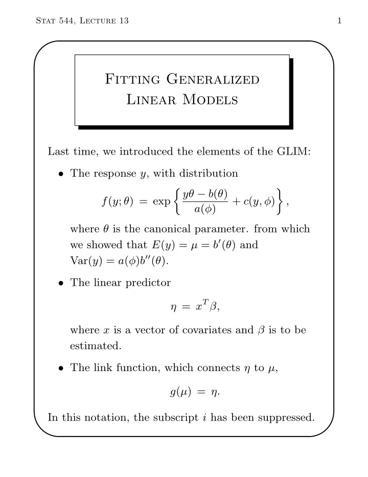
✬ ✩ Stat 544, Lecture 13 1 Fitting Generalized Linear Models Last time, we introduced the elements of the GLIM: • The response y , with distribution j yθ − b ( θ ) ff f ( y ; θ ) = exp + c ( y, φ ) , a ( φ ) where θ is the canonical parameter. from which we showed that E ( y ) = µ = b ′ ( θ ) and Var( y ) = a ( φ ) b ′′ ( θ ). • The linear predictor η = x T β, where x is a vector of covariates and β is to be estimated. • The link function, which connects η to µ , g ( µ ) = η. ✫ ✪ In this notation, the subscript i has been suppressed.

✬ ✩ Stat 544, Lecture 13 2 In many cases, a ( φ ) will have the form a ( φ ) = φ/w, where φ is the dispersion parameter and w is a known weight. Example: normal response. Under the normal model y ∼ N ( µ, σ 2 ), the log-density is − 1 2 σ 2 ( y − µ ) 2 − 1 2 πσ 2 ´ ` log f = 2 log yµ − µ 2 / 2 − y 2 2 σ 2 − 1 2 πσ 2 ´ ` = 2 log . σ 2 Therefore, the canonical parameter is θ = µ , and the remaining elements are b ( θ ) = µ 2 / 2 and φ = σ 2 , a ( φ ) = φ . In a heteroscedastic model y ∼ N ( µ, σ 2 /w ), where w is a known weight, we would have φ = σ 2 and a ( φ ) = φ/w . Example: binomial response. If y ∼ n − 1 Bin( n, π ), then the log-probability mass function is log f = log n ! − log( ny )! − log( n (1 − y ))! ✫ ✪ + ny log π + n (1 − y ) log(1 − π )

✬ ✩ Stat 544, Lecture 13 3 “ ” π y log + log(1 − π ) 1 − π = + c, 1 /n where c doesn’t involve π . Therefore, the canonical parameter is „ « π θ = log , 1 − π the b -function is “ 1 + e θ ” b ( θ ) = − log(1 − π ) = log , the dispersion parameter is φ = 1, and a ( φ ) = φ/n . Canonical link. We showed that the canonical parameter for y ∼ N ( µ, σ 2 ) is θ = µ , and the canonical parameter for ny ∼ Bin( n, π ) is θ = logit( π ). Notice that the most commonly used link function for a normal model is η = µ , and the most commonly used link function for the binomial model us η = logit( π ). This is no accident. When η = θ , we say that the model has a canonical link. Canonical links have some nice properties, which we will discuss. It is often convenient to use a canonical link. But convenience does not imply that the data actually ✫ ✪ conform to it. It will be important to check the

✬ ✩ Stat 544, Lecture 13 4 appropriateness of the link through diagnostics, whether or not the link is canonical. Fitting generalized linear models via Fisher scoring. ML estimation for β may be carried out via Fisher scoring, i − 1 β ( t +1) = β ( t ) + h − E l ′′ ( β ( t ) ) l ′ ( β ( t ) ) , where l is the loglikelihood function for the entire sample y 1 , . . . , y N . Temporarily changing the notation, we will now let l , l ′ and l ′′ denote the contribution of a single observation y i = y to the loglikelihood and its derivatives. We do this for simplicity, understanding that the corresponding functions for the entire sample are obtained by summing the contributions over the sample units i = 1 , . . . , N . Ignoring constants, the loglikelihood is l ( θ ; y ) = yθ − b ( θ ) . a ( φ ) The contribution of y = y i to the j th element of the ✫ ✪

✬ ✩ Stat 544, Lecture 13 5 score vector is „ ∂l «„ ∂θ «„ ∂η «„ ∂µ « ∂l ∂β j = . ∂θ ∂µ ∂η ∂β j The first factor is ∂θ = y − b ′ ( θ ) ∂l = y − µ a ( φ ) . a ( φ ) Because µ = b ′ ( θ ), the second factor is ∂θ 1 1 a ( φ ) ∂µ = b ′′ ( θ ) = V ( µ ) = Var( y ) , where V ( µ ) = b ′′ ( θ ) is the variance function that we discussed last time. The third factor, ∂µ/∂η , will depend on the link function. The fourth factor is ∂η/β j = x ij , where x ij is the j th element of the covariate vector x i = x for the i th observation. Putting it all together, we have „ ∂µ « ∂l y − µ ∂β j = x ij . Var( y ) ∂η If we are using the canonical link η = θ , then ∂µ/∂η = ∂µ/∂θ = b ′′ ( θ ), so the score becomes ∂l Var( y ) b ′′ ( θ ) x ij = y − µ y − µ ∂β j = a ( φ ) x ij . ✫ ✪ To find the expected second derivatives, we can use

✬ ✩ Stat 544, Lecture 13 6 the property »„ ∂l «„ ∂l ∂ 2 l „ « «– − E = E ∂β j ∂β k ∂β j ∂β k „ y − µ 2 „ ∂µ 2 « « = E x ij x ik Var( y ) ∂η 2 „ ∂µ « 1 = x ij x ik . Var( y ) ∂η With the canonical link, this becomes ∂ 2 l „ « = − b ′′ ( θ ) E a ( φ ) x ij x ik . ∂β j ∂β k But under the canonical link, the actual second derivative is „ ∂l «„ ∂θ ∂ 2 l « ∂ = ∂β j ∂β k ∂β k ∂θ ∂β j „ ∂l „ ∂θ «„ ∂ 2 l «„ ∂θ ∂ 2 θ «„ « « . = + ∂θ 2 ∂θ ∂β j ∂β k ∂β j ∂β k „ ∂ 2 l « x ij x ik . = 0 + ∂θ 2 Also, we saw last time that ∂ 2 l ∂θ 2 = − b ′′ ( θ ) a ( φ ) , ✫ ✪ so with the canonical link, the actual second

✬ ✩ Stat 544, Lecture 13 7 derivatives equal the observed second derivatives, and Fisher scoring is the same thing as Newton-Raphson. Under the canonical link, the second derivatives are constant with respect to the data y . Putting it together. For an arbitrary link, we have just shown that „ ∂µ « ∂l y − µ = x ij , ∂β j Var( y ) ∂η 2 ∂ 2 l „ « „ ∂µ « 1 − E = x ij x ik . ∂β j ∂β k Var( y ) ∂η It follows that the score vector for the entire data set y 1 , . . . , y N can be written as ∂l ∂β = X T A ( y − µ ) , where X = ( x 1 , . . . , x N ) T , » „ ∂µ i «– [Var( y i )] − 1 A = Diag , ∂η i „ ∂η i «– − 1 » = Diag Var( y i ) , ∂µ i and y and µ now denote the entire vectors ( y 1 , . . . , y N ) T , ✫ ✪ y =

✬ ✩ Stat 544, Lecture 13 8 ( µ 1 , . . . , µ N ) T . µ = The expected Hessian matrix becomes ∂ 2 l „ « = X T WX, − E ∂β∂β T where " 2 # „ ∂µ i « [Var( y i )] − 1 W = Diag ∂η i „ ∂η i 2 # − 1 " « = Diag Var( y i ) . ∂µ i An iteration of Fisher scoring is then ” − 1 β ( t +1) = β ( t ) + “ X T WX X T A ( y − µ ) , where W , A and µ are calculated from β ( t ) . Iteratively reweighted least squares. Recall that a heteroscedastic normal model is fit by weighted least squares (WLS), ” − 1 “ ˆ X T WX X T Wy, β = where y is the response and W is the diagonal matrix ✫ ✪ of weights, which is equivalent to OLS regression of

✬ ✩ Stat 544, Lecture 13 9 W 1 / 2 y on W 1 / 2 X . We can arrange the step of Fisher scoring to make it resemble WLS. First, rewrite it as ” − 1 h β ( t +1) = X T WXβ ( t ) + X T “ i X T WX A ( y − µ ) . Then note that Xβ = ( η 1 , . . . , η N ) T = η . Also, note that A and W are related by „ ∂η « A = W , ∂µ where ∂η/∂µ = Diag( ∂η i /∂µ i ). Therefore, we can write it as ” − 1 β ( t +1) = “ X T WX X T Wz, where „ ∂η « z = η + ( y − µ ) ∂µ ( z 1 , . . . , z N ) T , = where z i = η i + ( ∂η i /∂µ i )( y i − µ i ). In the GLIM literature, z i is often called the adjusted dependent variate or the working variate . Fisher scoring can therefore be regarded as iteratively reweighted least ✫ ✪ squares (IRWLS) carried out on a transformed version

✬ ✩ Stat 544, Lecture 13 10 of the response variable. At each cycle, we • use the current estimate for β to calculate a new working variate z and a new set of weights W , and then • regress z on X using weights W to get the updated β . Viewing Fisher scoring as IRWLS makes it easy to program this algorithm as a macro in any statistical package (even Minitab!) capable of WLS. Viewing Fisher scoring as IRWLS has an additional advantage: It provides an excellent basis for us to derive model-checking diagnostics. The diagnostics that are commonly used in regression—plotting residuals versus fitted values, leverage and influence measures, etc.—have obvious analogues in GLIM’s when we view the fitting procedure as IRWLS. Covariance matrix. The final value for ( X T WX ) − 1 upon convergence is the estimated covariance matrix for ˆ β . The diagonal elements of this matrix provide ✫ ✪

✬ ✩ Stat 544, Lecture 13 11 the squared SE’s for the estimated coefficients. What about the dispersion parameter? Recall that the variance of y i is usually of the form V ( µ i ) φ/w i , where V is the variance function, φ is the dispersion parameter, and w i is a known weight. In this case, φ cancels out of the IRWLS procedure and ˆ β itself is the same under any assumed value for φ . So, we could actually remove φ from the W matrix. But we have to be careful, because the assumed value for φ must be put back in to get a correct estimated covariance matrix for ˆ β . Example: Normal regression. Suppose that y i ∼ N ( µ i , σ 2 /w i ) where w i is a known weight, and let η i = g ( µ i ) = x T i β for some link function g . In this case, φ = σ 2 and the variance function is constant. If we use a log link, log µ i = x T i β, then ∂η i /∂µ i = 1 /µ i , the weight matrix is » w i µ 2 – i W = Diag , ✫ σ 2 ✪