Ferit Akova a,b in collaboration with Yuan Qi b , Bartek Rajwa c and - PowerPoint PPT Presentation
Ferit Akova a,b in collaboration with Yuan Qi b , Bartek Rajwa c and Murat Dundar a a Computer & Information Science Department, Indiana University Purdue University, Indianapolis (IUPUI) b Computer Science Department, Purdue University,
Ferit Akova a,b in collaboration with Yuan Qi b , Bartek Rajwa c and Murat Dundar a a Computer & Information Science Department, Indiana University – Purdue University, Indianapolis (IUPUI) b Computer Science Department, Purdue University, West Lafayette, IN c Discovery Park, Purdue University, West Lafayette, IN
Overview Semi-supervised learning and the fixed model assumption Gaussian assumption per class labeled unlabeled 2
Overview A new direction for Semi-supervised learning utilizes unlabeled data to improve learning even when labeled data is partially-observed uses self-adjusting generative models instead of fixed ones discovers new classes and new components of existing classes 3
Outline 1. Learning in Non-exhaustive Settings 2. Motivating Problems 3. Overview of the Proposed Approach 4. Partially-observed Hierarchical Dirichlet Processes 5. Illustration and Experiments 6. Conclusion and Future Work 4
Non-exhaustive Setting Training dataset is unrepresentative if the list of classes is incomplete, i.e., non-exhaustive Future samples of unknown classes will be misclassified (into one of the existing classes) with a probability one ill-defined classification problem! blue: known green & purple: unknown 5
What may lead to non-exhaustiveness? Some classes may not be in existence Classes may exist but may not be known Classes may be known but samples are unobtainable Exhaustive training data not realistic for many problems 6
Some Application Domains Classification of documents by topics research articles, web pages, news articles Image annotation Object categorization Bio-detection Hyperspectral image analysis 7
Biodetection Food Pathogens Acquired samples are from most prevalent classes High mutation rate, new classes A B can emerge anytime An exhaustive training library simply impractical Inherently non-exhaustive C D setting (A) Listeria monocytogenes 7644, (B) E. coli ETEC O25, (C)Staphylococcus aureus P103, (D)Vibrio cholerae O1E 8
Hyperspectral Data Analysis Military projects, GIS, urban planning, ... Physically inaccessible or dynamically changing areas Enemy territories, special military bases urban fields, construction areas Impractical to obtain an exhaustive training data 9
Semi-supervised Learning (SSL) Traditional approaches 1. self-training, 2. co-training, 3. transductive methods, 4. graph-based methods, 5. generative mixture models Unlabeled data improves classification under certain conditions, but primarily: model assumption matches the model generating the data Limited labeled data not only scarce, but usually data distribution not fully represented or maybe evolving 10
SSL in Non-exhaustive Settings A new framework for semi-supervised learning replaces the (brute-force fitting of a) fixed data model dynamically includes new classes/components classifies incoming samples more accurately A self-adjusting model to better accommodate unlabeled data 11
Our Approach in a Nutshell Classes as Gaussian mixture model (GMM) with unknown number of components Extension of HDP to dynamically model new components/classes Parameter sharing across inter- & intra-class components Collapsed Gibbs sampler for inference 12
Our Notation 13
DP, HDP Briefly… Dirichlet Process (DP): a nonparametric prior over the number of mixture components with base distribution G 0 and parameter α Hierarchical DP: models each group/class as a DP mixture and couples the G j ’s through a higher level DP 𝑦 𝑘𝑗 |𝜄 ~ 𝑞(⋅ |𝜄 𝑘𝑗 ) 𝑔𝑝𝑠 𝑓𝑏𝑑ℎ 𝑘, 𝑗 𝑘𝑗 𝜄 𝑘𝑗 |𝐻 ~ 𝐻 𝑘 𝑔𝑝𝑠 𝑓𝑏𝑑ℎ 𝑘, 𝑗 𝑘 𝐻 𝑘 |𝐻 0 , 𝛽 ~ 𝐸𝑄(𝐻 0 , 𝛽) 𝑔𝑝𝑠 𝑓𝑏𝑑ℎ 𝑘 𝐻 0 |𝐼, 𝛿 ~ 𝐸𝑄(𝐼, 𝛿) α controls the prior probability of a new component 14
Modeling with HDP Chinese Restaurant Franchise (CRF) analogy Restaurants correspond to classes, tables to mixture components and dishes in the “global menu” to unique parameters First customer at a table orders a dish Popular dishes more likely to be chosen Role of γ in picking a new dish from the menu 15
Conditional Priors in CRF Seating customers and assigning dishes to tables t ji – index of the table for customer i in restaurant j k jt – index of the dish served at table t in restaurant j 𝑛 𝑘. 𝑜 𝑘𝑢 𝛽 𝑜 𝑘 + 𝛽 𝜀 𝑢 𝑜 𝑘 + 𝛽 𝜀 𝑢 𝑜𝑓𝑥 + 𝑢 𝑘𝑗 |𝑢 𝑘1 , … , 𝑢 𝑘,𝑗−1 , 𝛽 ~ 𝑢=1 𝐿 𝛿 𝑛 .𝑙 𝑛 .. + 𝛿 𝜀 𝑙 𝑛 .. + 𝛿 𝜀 𝑙 𝑜𝑓𝑥 + 𝑙 𝑘𝑢 |𝑙 𝑘1 , … , 𝑙 𝑘,𝑢−1 , 𝛿 ~ 𝑙=1 16
Inference in HDP Gibbs sampler to iteratively sample the indicator variables for tables and dishes given the state of all others 𝐾 𝐾 𝑜 𝑘 𝑛 𝑘. 𝐿 , 𝐥 = , 𝜚 = 𝜚 𝑙 𝑙=1 𝐮 = 𝑢 𝑘𝑗 𝑗=1 𝑙 𝑘𝑢 𝑢=1 𝑘=1 𝑘=1 Conjugate pair of H and P(.| φ ) allows for integrating out φ to obtain a collapsed version α and γ also sampled in each sweep based on number of tables and dishes, respectively. (Escobar & West, 1994) 17
Gibbs Sampler for t and k Conditional weighted by number of samples Joint probability weighted by number of components 18
Defining Partially-observed Setting Observed classes/subclasses: Those initially available in the training library. Unobserved classes/subclasses: Those not represented in the training library New classes: classes discovered online, verified offline limited to a single component until manual verification 19
HDP in a Partially-observed Setting Two tasks: Inferring component membership of labeled samples 1. Inferring both the group and component membership 2. of unlabeled samples Unlabeled samples evaluated for all existing components 20
Inference in Partially-observed HDP Updated Gibbs sampling inference for t ji 21
Inference in Partially-observed HDP Updated inference for k jt for existing and new classes 22
Gaussian Mixture Model Data Σ 0 , 𝑛, 𝜈 0 , 𝜆 estimated from labeled data by Empirical Bayes 23
Inference from GMM Data 24
Parameter Sharing in a GMM 25
Illustrative Example 3 classes as a mixture of 3 components 110 samples in each component, 10 randomly selected as labeled 100 considered as unlabeled Covariance matrices from a set of 5 templates 26
Illustrative Example 1 Standard HDP using only labeled data 2 A fixed generative model assigning full weight to labeled samples and reduced weight to unlabeled ones. 3 SA-SSL using labeled and unlabeled data with parameter sharing 27
Experiments - Evaluated Classifiers Baseline supervised learning methods using only labeled data Naïve-Bayes (SL-NB), Maximum likelihood (SL-ML), expectation maximization (SL-EM) Benchmark semi-supervised learning methods Self-training with base learners ML and NB (SELF) Co-training with base learners ML and NB (CO-TR) SSL-EM: Standard generative model approach SSL-MOD: EM based approach with unobserved class modeling SA-SSL: Proposed Self-adjusting SSL approach 28
Experiments – Classifier Design Split available labeled data into train , unlabeled and test Stratified sampling to represent each class proportionally Consider some classes “ unobserved ” moving their samples from training set to unlabeled set Non-exhaustive training set, exhaustive unlabeled and test sets 29
Experiments – Evaluation Overall classification accuracy Average accuracies on observed and unobserved classes Newly created components associated with unobserved classes according to majority of samples Repeated with 10 random test/train/unlabeled splits 30
Remote Sensing 31
Remote Sensing Results 20 components and 10 unique covariance matrices in total Two to three components per each of the 8 classes Half of the components shares covariance matrices 32
Pathogen Detection Experiment Total of 2054 samples from 28 bacteria classes Each class contains between 40 to 100 samples 22 feature samples 4 classes made unobserved, 24 classes remains observed 30% as test , 20% as train and remaining 50% as unlabeled Method Acc Acc-O Acc-U Totally 180 components, 150 SA-SSL 0.81 0.80 0.84 unique covariance matrices SSL-EM 0.64 0.75 0 Five to six components SSL-MOD 0.67 0.74 0.26 per each class SELF 0.59 0.70 0 One sixth of the components CO-TR 0.60 0.72 0 shared parameter with others SL-ML 0.62 0.73 0 SL-NB 0.52 0.62 0 SL-EM 0.30 0.35 0 33
Recap of the Contributions A new approach to learning with a non-exhaustively defined labeled data set A unique framework to utilize unlabeled samples in partially-observed semi-supervised settings 1) Extension of HDP model to entertain unlabeled data and to discover & recover new classes 2) Fully Bayesian treatment of mixture components to allow parameter sharing across different components addresses the curse of dimensionality a) connects observed classes with unobserved ones b) 34
Recommend
More recommend
Explore More Topics
Stay informed with curated content and fresh updates.
