Faster Algorithms for Next Breakpoint and Max Value for Parametric - PDF document
Faster Algorithms for Next Breakpoint and Max Value for Parametric Global Minimum Cuts ene Aissi 1 , S. Thomas McCormick 2 , and Maurice Queyranne 2 Hass` 1 Paris Dauphine University. aissi@lamsade.dauphine.fr 2 Sauder School of Business at the
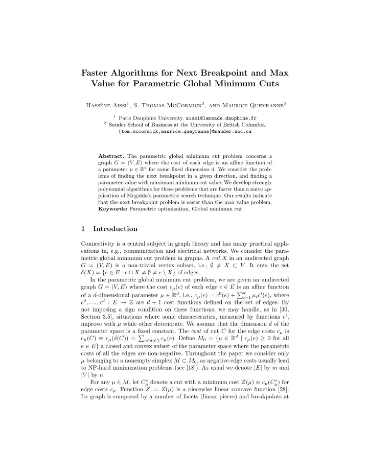
Faster Algorithms for Next Breakpoint and Max Value for Parametric Global Minimum Cuts ene Aissi 1 , S. Thomas McCormick 2 , and Maurice Queyranne 2 Hass` 1 Paris Dauphine University. aissi@lamsade.dauphine.fr 2 Sauder School of Business at the University of British Columbia. { tom.mccormick,maurice.queyranne } @sauder.ubc.ca Abstract. The parametric global minimum cut problem concerns a graph G = ( V, E ) where the cost of each edge is an affine function of a parameter µ ∈ R d for some fixed dimension d . We consider the prob- lems of finding the next breakpoint in a given direction, and finding a parameter value with maximum minimum cut value. We develop strongly polynomial algorithms for these problems that are faster than a naive ap- plication of Megiddo’s parametric search technique. Our results indicate that the next breakpoint problem is easier than the max value problem. Keywords: Parametric optimization, Global minimum cut. 1 Introduction Connectivity is a central subject in graph theory and has many practical appli- cations in, e.g., communication and electrical networks. We consider the para- metric global minimum cut problem in graphs. A cut X in an undirected graph G = ( V, E ) is a non-trivial vertex subset, i.e., ∅ � = X ⊂ V . It cuts the set δ ( X ) = { e ∈ E : e ∩ X � = ∅ � = e \ X } of edges. In the parametric global minimum cut problem, we are given an undirected graph G = ( V, E ) where the cost c µ ( e ) of each edge e ∈ E is an affine function of a d -dimensional parameter µ ∈ R d , i.e., c µ ( e ) = c 0 ( e ) + � d i =1 µ i c i ( e ), where c 0 , . . . , c d : E → Z are d + 1 cost functions defined on the set of edges. By not imposing a sign condition on these functions, we may handle, as in [30, Section 3.5], situations where some characteristics, measured by functions c i , improve with µ while other deteriorate. We assume that the dimension d of the parameter space is a fixed constant. The cost of cut C for the edge costs c µ is e ∈ δ ( C ) c µ ( e ). Define M 0 = { µ ∈ R d | c µ ( e ) ≥ 0 for all c µ ( C ) ≡ c µ ( δ ( C )) = � e ∈ E } a closed and convex subset of the parameter space where the parametric costs of all the edges are non-negative. Throughout the paper we consider only µ belonging to a nonempty simplex M ⊂ M 0 , as negative edge costs usually lead to NP-hard minimization problems (see [18]). As usual we denote | E | by m and | V | by n . For any µ ∈ M , let C ∗ µ denote a cut with a minimum cost Z ( µ ) ≡ c µ ( C ∗ µ ) for edge costs c µ . Function Z := Z ( µ ) is a piecewise linear concave function [28]. Its graph is composed by a number of facets (linear pieces) and breakpoints at
Hass` 2 ene Aissi, S. Thomas McCormick, and Maurice Queyranne which d facets meet. In order to avoid dealing with a trivial problem, Z is as- sumed to have at least one breakpoint. The maximum number of facets (linear pieces) of the graph of Z is called the combinatorial facet complexity of Z . Mul- muley [23, Theorem 3.10] considers the case d = 1 and gives a super-polynomial bound on the combinatorial facet complexity of the global minimum cut prob- lem. In [3, Theorem 4], the authors extended this result to a constant dimension m d n 2 log d − 1 n � � d and give a strongly polynomial bound O . By combining this result with several existing computational geometry algorithms, the authors give an O ( m d ⌊ d − 1 2 ⌋ n 2 ⌊ d − 1 2 ⌋ log ( d − 1) ⌊ d − 1 2 ⌋ + O (1) n ) time algorithm for constructing function Z for general d , and a O ( mn 4 log n + n 5 log 2 n ) algorithm when d = 1. In the particular case where cost functions c 0 , . . . , c d are nonnegative, Karger [15] � n d +2 � gives a significantly tighter bound O on the combinatorial facet complex- ity and shows that function Z can be computed using a randomized algorithm in � n 2 d +2 log n � O time. These results are summarized in rows 5 and 6 of Table 1. In this paper, we consider the following parametric problems: P NB ( M ) Given a polyhedron M ⊂ R d , a value µ 0 ∈ M ⊂ R d , and a direction ν ∈ Z d . Find the next breakpoint µ NB ∈ M of Z after µ 0 in direction ν , if any. P max ( M ) Given a polyhedron M ⊂ R d , find a value µ ∗ ∈ M such that Z ( µ ∗ ) = max µ ∈ M Z ( µ ). In contrast to P max ( M ), P NB ( M ) is a one-dimensional parametric optimiza- tion problem as it considers the restriction of function Z to some direction ν ∈ Z d . This problem corresponds to the ray shooting problem which is a stan- dard topic in sensitivity analysis [11, Section 30.3] to identify ranges of opti- mality and related quantities. Given λ � 0, the cost c µ 0 + λν of each edge e ∈ E in the direction ν is defined by c µ 0 + λν ( e ) = c 0 ( e ) + � d i =1 ( µ 0 i + λν i ) c i ( e ). Let c 0 ( e ) = c 0 ( e ) + � d c 1 ( e ) = � d i =1 µ 0 c i ( e ) and ¯ i =1 ν i c i ( e ). The edge costs can be ¯ c 0 ( e ) + λ ¯ c 1 ( e ). For any cut ∅ � = C ⊂ V , its cost for the rewritten as c µ 0 + λν ( e ) = ¯ c 0 ( C )+ λ ¯ c 1 ( C ) of variable λ . For any edge costs c µ 0 + λν is a function c µ 0 + λν ( C ) = ¯ λ ≥ 0 let Z ′ ( λ ) = Z ′ ( µ 0 + λν, ν ) denote the right derivative of Z ( µ 0 + λν ) in direc- tion ν at λ . If the next breakpoint µ NB exists, define λ NB by µ NB = µ 0 + λ NB ν , and let C ∗ µ NB denote an optimal cut for edge costs c µ NB ( e ) defining the slope Z ′ ( λ NB ). P max ( M ) arises in the context of network reinforcement problem. Consider the following 2-player game of reinforcing a graph against an attacker. Given a graph G = ( V, E ) where each edge e ∈ E has a capacity c 0 ( e ), the Graph player wants to reinforce the capacities of the edges in E by buying d + 1 resources subject to a budget B . The Graph player can spend $ µ i � 0 on each resource i to increase the capacities of all edges to c µ ( e ) = c 0 ( e ) + � d +1 i =1 µ i c i ( e ), where all functions c i are assumed to be non-negative. The Attacker wants to remove some edges of E in order to cut the graph into two pieces at a minimum cost. Therefore, these edges correspond to an optimal cut δ ( C ∗ µ ) and their removal cost is Z ( µ ). The Graph player wants to make it as expensive as possible for the Attacker to
Faster Algorithms for Parametric Global Minimum Cut Problems 3 cut the graph, and so he wants to solve P max . It is optimal for the Graph player to spend all the budget, and thus to spend µ d +1 = B − � d i =1 µ i on resource d + 1. Therefore, the cost of removing edge e as a function of the amounts spent on the first d resources is c µ ( e ) = c 0 ( e )+ � d B − � d c d +1 ( e ) = i =1 µ i c i ( e )+ � � i =1 µ i + � d � c 0 ( e ) + Bc d +1 ( e ) � � c i ( e ) − c d +1 ( e ) � . Note that c i ( e ) − c d +1 ( e ) may be i =1 µ i negative. This application illustrates how negative parametric edge costs may arise even when all original data are non-negative. Clearly problems P max ( M ) and P NB ( M ) can be solved by constructing func- tion Z . However, the goal of this paper is to give much faster strongly polynomial algorithms for these problems without explicitly constructing the whole function Z . 1.1 Related works The results mentioned in this section are summarized in the first four rows of Table 1. We concentrate on strongly polynomial bounds here as is the case in most of the literature, but see Section 1.3 for one case where there is a potentially faster weakly polynomial bound. Problem Deterministic Randomized Non-param Global MC [24, 31] O ( mn + n 2 log n ) [14] ˜ O ( m ) ([16] ˜ O ( n 2 )) 3 [25] O ( n 4 ) [16] ˜ O ( n 2 ) All α -approx for α < 4 Megiddo P NB ( ∼ d = 1) [31] O ( n 5 log n ) [32, 16] O ( n 2 log 5 n ) Megiddo P max ( ∼ gen’l d ) [31] O ( n 2 d +3 log d n ) [32, 16] O ( n 2 log 4 d +1 n ) All of Z ( µ ) for d = 1 [3] O ( mn 4 log n + n 5 log 2 n ) [15] O ( n 4 log n ) [15] O ( n 2 d +2 log n ) All of Z ( µ ) for gen’l d [3] [big] This paper P NB ( ∼ d = 1) [24, 31] O ( mn + n 2 log n ) [13] O ( n 2 log 3 n ) This paper P max ( ∼ gen’l d ) O ( n 4 log d − 1 n ) ??? Table 1. New results in this paper are in red. Compare these to the non-parametric lower bounds in green, and the various upper bounds in blue. The standard (non-parametric) global minimum cut minimum cut is a special case of the parametric global minimum cut, i.e., for some fixed value µ ∈ M . Nagamochi and Ibaraki [24] and Stoer and Wagner [31] give a deterministic algorithm for this problem that runs in O ( mn + n 2 log n ) time. Karger and Stein [16] give a faster randomized algorithm that runs in ˜ O ( n 2 ) time. Karger [14] improves the running time and give an ˜ O ( m ) time algorithm. Given α > 1, a cut is called α -approximate if its cost is at most at factor of α larger than the optimal value. A remarkable property of the global minimum cut problem is that there exists a strongly polynomial number of near-optimal cuts. Karger [14] showed that the number of α -approximate cuts is O ( n ⌊ 2 α ⌋ ). Nagamochi et al. [26] give a deterministic O ( m 2 n + mn 2 α ) time algorithm for 4 enumerating them. For the particular case 1 < α < 3 , they improved this
Recommend
More recommend
Explore More Topics
Stay informed with curated content and fresh updates.


