Fast sampling and counting -SAT solutions in the local lemma regime - PowerPoint PPT Presentation

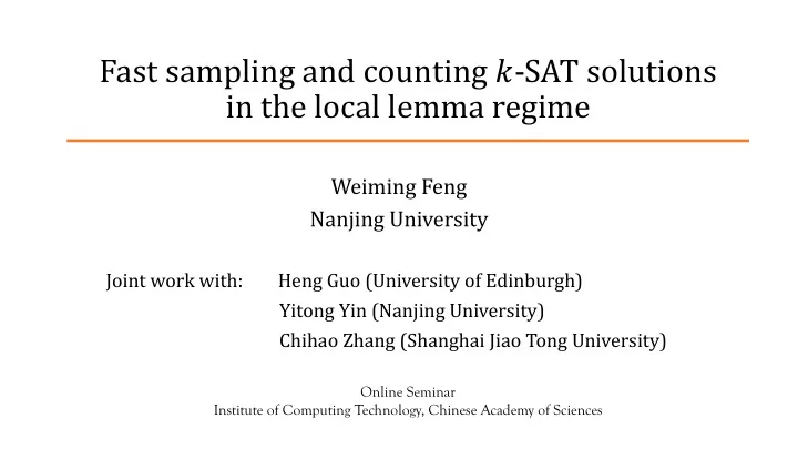
Fast sampling and counting 𝑙 -SAT solutions in the local lemma regime Weiming Feng Nanjing University Joint work with: Heng Guo (University of Edinburgh) Yitong Yin (Nanjing University) Chihao Zhang (Shanghai Jiao Tong University) Online Seminar Institute of Computing Technology, Chinese Academy of Sciences

Conjunctive normal form (CNF) • Instance : a formula Φ = (𝑊, 𝐷) , for example clause Φ = 𝑦 ! ∨ ¬𝑦 " ∨ 𝑦 # ∧ 𝑦 ! ∨ 𝑦 " ∨ 𝑦 $ ∧ 𝑦 # ∨ ¬𝑦 $ ∨ ¬𝑦 % 𝑊 = {𝑦 ! , 𝑦 " , 𝑦 # , 𝑦 $ , 𝑦 % }: set of Boolean variables; 𝐷 : set of clauses. • SAT solutions : an assignment of variables in 𝑊 s.t. 𝚾 = true . • Fundamental computational tasks for CNF formula: • Decision : Does SAT solution exist? NP-Complete problem [Cook 1971, Levin 1973]. • Counting : How many SAT solutions? #P-Complete problem [Valiant 1979].

𝑙, 𝑒 -CNF formula Φ = (𝑊, 𝐷) • Each clause contains 𝑙 Boolean variables. • Each variable belongs to at most 𝑒 clauses, e.g. max degree ≤ 𝒆 . Example: (3,2)-CNF formula 𝑦 ! ∨ ¬𝑦 " ∨ 𝑦 # ∧ 𝑦 ! ∨ 𝑦 " ∨ 𝑦 $ ∧ 𝑦 # ∨ ¬𝑦 $ ∨ ¬𝑦 % Lovász Local Lemma (LLL) Suppose a ( 𝑙, 𝑒 )-CNF formula satisfies 𝒍 ≳ 𝐦𝐩𝐡 𝒆 (𝑙 ≥ log 𝑒 + log 𝑙 + 𝐷) . Existence [Erdős, Lovász, 1975] • If each variable takes a value in {true,false} uniformly and independently !" 1 Pr all clauses are satis?ied ≥ 1 − > 0, 2𝑒𝑙 which implies the 𝑙 -SAT solution must exist ; Construction [Moser, Tardos, 2010] • a 𝑙 -SAT solution can be constructed in expected time 𝑃 𝑜𝑒𝑙 .

Sampling & counting 𝑙 -SAT solutions • Input: a 𝑙, 𝑒 -CNF formula Φ = (𝑊, 𝐷) with 𝑊 = 𝑜 , and error bound 𝜗 > 0 . • Almost uniform sampling: generate a random SAT solution 𝑌 ∈ true, false % s.t. the total variation distance is at most 𝜗 , 𝑒 &% 𝑌, 𝜈 = 1 ) Pr 𝑌 = 𝜏 − 𝜈(𝜏) ≤ 𝜗 2 # '∈ true,false 𝜈 : the uniform distribution of all 𝑙 -SAT solutions.

Sampling & counting 𝑙 -SAT solutions • Input: a 𝑙, 𝑒 -CNF formula Φ = (𝑊, 𝐷) with 𝑊 = 𝑜 , and error bound 𝜗 > 0 . • Almost uniform sampling: generate a 𝑙 -SAT solution 𝑌 ∈ true, false % s.t. the total variation distance 𝑒 &% 𝑌, 𝜈 ≤ 𝜗, 𝜈 : the uniform distribution of all 𝑙 -SAT solutions. • Approximate counting: estimate the number of 𝑙 -SAT solutions, e.g. output 1 − 𝜗 𝑎 ≤ 9 𝒂 ≤ 1 + 𝜗 𝑎, 𝑎 = the number of 𝑙 -SAT solutions. Self-reduction [Jerrum, Valiant, Vazirani 1986] Almost Uniform Approximate Sampling Counting Simulated annealing [Štefankovič et al. 2009]

Work Regime Running time/lower bound Technique Monotone CNF [1] Markov chain Monte Carlo poly 𝑒𝑙 𝑜 log 𝑜 Hermon et al.’19 𝑙 ≳ 2 log 𝑒 (MCMC) 𝑡 ≥ min log 𝑒𝑙 , 𝑙/2 [2] poly 𝑒𝑙 𝑜 Guo et al.’17 Partial rejection sampling 𝑙 ≳ 2 log 𝑒 𝑜 $%&'(!)) Moitra’17 𝑙 ≳ 60 log 𝑒 Linear programming NP-hard Bezáková et al.’15 𝑙 ≤ 2 log 𝑒 − 𝐷 - Table: previous results for sampling SAT solutions of 𝑙, 𝑒 -CNF formulas [1] Monotone CNF: all variables appear positively, e.g. 𝛸 = 𝑦 ! ∨ 𝑦 " ∨ 𝑦 # ∧ 𝑦 " ∨ 𝑦 $ ∨ 𝑦 % ∧ 𝑦 # ∨ 𝑦 $ ∨ 𝑦 & . [2] s: two dependent clauses share at least 𝑡 variables. Open Problem: Can we sample general 𝑙, 𝑒 -CNF solutions such that the threshold down to 𝑙 ≳ 2 log 𝑒 ; • the running time poly(𝑒𝑙) 1 𝑃 (𝑜) . •

Our result Work Regime Running time/lower bound Technique Monotone CNF poly 𝑒𝑙 𝑜 log 𝑜 Hermon et al.’19 MCMC 𝑙 ≳ 2 log 𝑒 𝑡 ≥ min log 𝑒𝑙 , 𝑙/2 poly 𝑒𝑙 𝑜 Guo et al.’17 Partial rejection sampling 𝑙 ≳ 2 log 𝑒 𝑜 $%&'(!)) Moitra’17 𝑙 ≳ 60 log 𝑒 Linear programming NP-hard Bezáková et al.’15 𝑙 ≤ 2 log 𝑒 − 𝐷 - ; 𝒍 ≳ 𝟑𝟏 𝐦𝐩𝐡 𝒆 𝑷(𝒆 𝟑 𝒍 𝟒 𝒐 𝟐.𝟏𝟏𝟏𝟏𝟏𝟐 ) This work MCMC Table: results for sampling SAT solutions of 𝑙, 𝑒 -CNF formulas

Main theorem (this work) For any sufficiently small 𝜂 < 2 EFG , any (𝑙, 𝑒) -CNF formula satisfying 𝑙 ≥ 20 log 𝑒 + 20 log 𝑙 + 3 log 1 𝜂 , • sampling algorithm (main algorithm) 𝑃 𝑒 F 𝑙 H 𝑜 IJK ; draw almost uniform random 𝑙 -SAT solution in time D • counting algorithm (by simulated annealing reduction) 𝑃 𝑒 H 𝑙 H 𝑜 FJK ; count #𝑙 -SAT solutions approximately in time D

Classic Glauber dynamics (Gibbs sampling) Start from an arbitrary solution 𝑍 ∈ 𝑈, 𝐺 % ; 𝑦 $ 𝑦 ! true For each 𝑢 from 1 to 𝑈 do 𝑦 % 𝑦 " 𝑦 ' false • Pick 𝑤 ∈ 𝑊 uniformly at random; 𝑦 & 𝑦 # • Resample 𝑍 N ∼ (⋅∣ 𝑍 %\N ) ; (𝑦 ! ∨ ¬𝑦 " ∨ 𝑦 # ) ∧ (𝑦 " ∨ 𝑦 ' ∨ 𝑦 % ) ∧ (𝑦 $ ∨ ¬𝑦 % ∨ 𝑦 & )

Classic Glauber dynamics (Gibbs sampling) Start from an arbitrary solution 𝑍 ∈ 𝑈, 𝐺 % ; 𝑦 $ 𝑦 ! true For each 𝑢 from 1 to 𝑈 do 𝑦 % 𝑦 " 𝑦 ' false • Pick 𝑤 ∈ 𝑊 uniformly at random; 𝑦 & 𝑦 # • Resample 𝑍 N ∼ (⋅∣ 𝑍 %\N ) ; (𝑦 ! ∨ ¬𝑦 " ∨ 𝑦 # ) ∧ (𝑦 " ∨ 𝑦 ' ∨ 𝑦 % ) ∧ (𝑦 $ ∨ ¬𝑦 % ∨ 𝑦 & )

Classic Glauber dynamics (Gibbs sampling) Start from an arbitrary solution 𝑍 ∈ 𝑈, 𝐺 % ; 𝑦 $ 𝑦 ! true For each 𝑢 from 1 to 𝑈 do 𝑦 % 𝑦 " 𝑦 ' T/F? false • Pick 𝑤 ∈ 𝑊 uniformly at random; 𝑦 & 𝑦 # • Resample 𝑍 N ∼ 𝜈 N (⋅∣ 𝑍 %\N ) ; (𝑦 ! ∨ ¬𝑦 " ∨ 𝑦 # ) ∧ (𝑦 " ∨ 𝑦 ' ∨ 𝑦 % ) ∧ (𝑦 $ ∨ ¬𝑦 % ∨ 𝑦 & )

Classic Glauber dynamics (Gibbs sampling) Start from an arbitrary solution 𝑍 ∈ 𝑈, 𝐺 % ; 𝑦 $ 𝑦 ! true For each 𝑢 from 1 to 𝑈 do 𝑦 % 𝑦 " 𝑦 ' F! false • Pick 𝑤 ∈ 𝑊 uniformly at random; 𝑦 & 𝑦 # • Resample 𝑍 N ∼ 𝜈 N (⋅∣ 𝑍 %\N ) ; (𝑦 ! ∨ ¬𝑦 " ∨ 𝑦 # ) ∧ (𝑦 " ∨ 𝑦 ' ∨ 𝑦 % ) ∧ (𝑦 $ ∨ ¬𝑦 % ∨ 𝑦 & )

Connectivity barrier (toy example) • (𝑙, 𝑒) -CNF formula Φ = (𝑊, 𝐷) with 𝑊 = 𝑦 I , 𝑦 F , … 𝑦 P : Φ = 𝐷 I ∧ 𝐷 F ∧ ⋯ ∧ 𝐷 P . 𝐷 I = (¬𝑦 I ∨ 𝑦 F ∨ 𝑦 H ∨ ⋯ ∨ 𝑦 P ) forbids 100 … 0 𝐷 F = (𝑦 I ∨ ¬𝑦 F ∨ 𝑦 H ∨ ⋯ ∨ 𝑦 P ) forbids 010 … 0 𝐷 P = (𝑦 I ∨ 𝑦 F ∨ 𝑦 H ∨ ⋯ ∨ ¬𝑦 P ) forbids 000 … 1 • Any assignment 𝑌 ∈ 0,1 % with 𝑌 I = 1 is infeasible. • All false solution 𝟏 is disconnected with others. 10…0 Other Solutions 00…0 01…0 00…1

“the solution space (and hence the natural Markov chain) is not connected” • Glauber dynamics : random walk over solution space via local update. • Local Markov chain : one of the most fundamental approach for sampling: uniform graph coloring weighted matching/independent set Ising/spin system bases of a matroid We are here ！ rapid mixing not mixing slow mixing For sampling CNF solutions, the MCMC approach meets the connectivity barrier . Mathematics and Computation [Wigderson’19]

Bypass the connectivity barrier Work Regime Running time Technique Monotone CNF Hermon et monotone CNF poly 𝑒𝑙 𝑜 log 𝑜 MCMC al.’19 𝑙 ≳ 2 log 𝑒 𝑡 ≥ min log 𝑒𝑙 , 𝑙/2 Guo, Jerrum, Partial rejection heavy intersection poly 𝑒𝑙 𝑜 Liu’17 𝑙 ≳ 2 log 𝑒 sampling 𝑜 !"#$(&') constant 𝒆 and 𝒍 Moitra’17 𝑙 ≳ 60 log 𝑒 Linear programming Non-MCMC approach Technique Motivation: Can MCMC approach bypass the connectivity barrier ?

Our technique: projection Source: https://www.shadowmatic.com/presskit/images/IMG_0650.png Projecting from a high dimension to a lower dimension to improve connectivity

Construct a good subset of variables 𝑁 ⊆ 𝑊 Run Glauber dynamics on projected distribution 𝜈 + to draw sample 𝑌 ∼ 𝜈 + Start from a uniform random 𝑌 ∈ true ,false ) ; For each 𝑢 from 1 to 𝑈 Pick a variable 𝑤 ∈ 𝑁 uniformly at random; • 𝒘 Resample 𝑌 * ∼ 𝜈 * (⋅ |𝑌 )\* ) ; • Return 𝑌 ∈ true ,false ) . T/F? Draw sample 𝑍 ∼ 𝜈 ,\+ (⋅ |𝑌) from the conditional distribution There exists an efficiently constructible subset 𝑁 ⊆ 𝑊 such that: computing exact distr. the Glauber dynamics on 𝜈 + is rapidly mixing , • can be #P-hard the Glauber dynamics on 𝜈 + can be implemented efficiently (draw 𝑌 . ∼ 𝜈 . (⋅ |𝑌 +\. ) ), • sampling assignment for 𝑊\𝑁 can be implemented efficiently (draw 𝑍 ∼ 𝜈 ,\+ (⋅ |𝑌) ). •

Construct a good subset of variables 𝑁 ⊆ 𝑊 Run Glauber dynamics on projected distribution 𝜈 + to draw sample 𝑌 ∼ 𝜈 + Start from a uniform random 𝑌 ∈ true ,false ) ; For each 𝑢 from 1 to 𝑈 Pick a variable 𝑤 ∈ 𝑁 uniformly at random; • 𝒘 Resample 𝑌 * ∼ 𝜈 * (⋅ |𝑌 )\* ) ; • Return 𝑌 ; T/F? Draw sample 𝑍 ∼ 𝜈 ,\+ (⋅ |𝑌) from the conditional distribution Our Tasks : Construct such a good subset 𝑁 ⊆ 𝑊 . • Show that the Glauber dynamics on 𝜈 + is rapidly mixing . • Given assignment on 𝑁 , draw samples efficiently from the conditional distribution. •