Fast Object Distribution Andrew Willmott Maxis, Electronic Arts - PowerPoint PPT Presentation
Fast Object Distribution Andrew Willmott Maxis, Electronic Arts Distributing Objects Goal: Place objects over an area Vary attributes (colour, size, etc.) Lots and lots of solutions Pseudo Random: LCG, Mersenne Twister Dart
Fast Object Distribution Andrew Willmott Maxis, Electronic Arts
Distributing Objects • Goal: Place objects over an area • Vary attributes (colour, size, etc.) • Lots and lots of solutions – Pseudo Random: LCG, Mersenne Twister – Dart throwing – Blue noise (Ostromoukhov et al.) – Wang tiles (Hall and Oates)
Our Constraints • Fast! (Game use) • Low memory (Low memory -> Fast) • Re-produceable • Control – Position – Orientation, Colour, Alpha, etc. – Density
Summary • Use Halton Sequence to generate N samples • Make it incremental for speed reasons • Use i / N as a magic number – To index attribute tables – To perform rejection sampling against maps • (You may leave now)
Halton Sequence • Basic idea: take the sample count in base b , and digit reverse it • In binary: 0 -> 0.0 1 -> 0.1 2 -> 0.01 3 -> 0.11 4 -> 0.001 5 -> 0.101 6 -> 0.011 7 -> 0.111
Halton Sequence • Extends to higher dimensions • Use base 3, 5, 7... to avoid correlation 20 100 500
Why Halton? • Ensures samples are well-spaced • It is extendable – Later samples in the sequence fill in between previous samples • It’s simple: no subdivision, spatial data structures, no state...
But • Too expensive for our purpose – Requires digit reversal of base 2, 3, 5 (3D) numbers – log_b(x) with divides in inner loop – Problem: Recalculate from scratch for each sample • Could use look-up tables – But that’s expensive too, for large tables – Also imposes an upper sample count limit
Incremental Halton Sequence • What changes between H n and H n+1 ? • For base 2: – Bottom m bits, depending on carry propagation – Each bit x that flips adds +-2 -x – So, form the difference, XOR( n, (n+1)) – Adjust H n accordingly • Expected iterations: 2
Incremental: Other Bases • Store count in BC<B> form. – Base 3 = 2 bits per digit, Base 5 = 3 bits per digit • As we manually propagate the carry, adjust H_n accordingly, either -(b-1)b -x , or + b -x • Expected carries/iterations – base 3 = 1.5, base 5 = 1.25
Choosing Attributes • Orientation, colour, transparency, size • Our usual approach: Data-drive from table – index with e.g. particle age (0-1) – or random number • New approach – i is sample number, use i / N to index – Areas well apart in the curve correspond to well- separated objects
Attribute Tables • Colour: 0 1 Random Selection • Size: • Rotation:
Attribute Tables i / N • Colour: 0 1 • Size: • Rotation:
Advantages • More controllable • As well as weighting, curve is controlling effect over distance – Red boxes farthest from yellow boxes • Curves are correlated too – Big yellow boxes, small red boxes
Object Nesting • Can apply the same technique to different model types • Allow artist control over where range starts • Subsequent types “fill in” without collision
Large Trees
Medium Trees
Bushes
Object Density Control • Want control either by image map or procedural map • Either may be game-affected, so minimal pre- processing desirable • Key observation: – As sample count increases, samples fill in between previous samples – Thus can affect overall density by varying N
Density Control • Can achieve the same effect locally by dropping out samples larger than a given cutoff N , depending on a local density control value • This reduces to: f ( p i ) < i / N : reject • ( p is sample i ’s position, f is density function)
Density Map
Distribution
Density Map
Distribution
Images
Images
Questions?
Recommend
More recommend
Explore More Topics
Stay informed with curated content and fresh updates.
