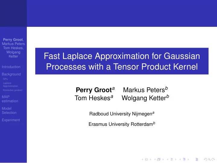
Fast Laplace Approximation for Gaussian Ketter Processes with a - PowerPoint PPT Presentation

Perry Groot , Markus Peters Tom Heskes, Wolgang Fast Laplace Approximation for Gaussian Ketter Processes with a Tensor Product Kernel Introduction Background GPs Laplace Approximation Perry Groot a Markus Peters b Kronecker product Tom Heskes a Wolgang Ketter b MAP estimation Model Selection Radboud University Nijmegen a Experiment Erasmus University Rotterdam b

Introduction Perry Groot , Markus Peters Tom Heskes, Gaussian process models Wolgang Ketter + rich, principled Bayesian framework Introduction - scalability O ( N 3 ) Background Approaches addressing scalability GPs Laplace Approximation approximations / subset selection O ( M 2 N ) Kronecker product exploit additional structure MAP estimation Tensor product kernels Model Selection + Efficient use of Kronecker products on grid data - Limited to standard regression, since Experiment if K = Q Λ Q T then ( K + σ 2 I ) − 1 y = Q ( Λ + σ 2 I ) − 1 Q T y .

Gaussian Processes Perry Groot , Markus Peters A Gaussian process (GP) is collection of random variables Tom Heskes, Wolgang with the property that the joint distribution of any finite Ketter subset is a Gaussian. Introduction Background GPs A GP specifies a probability distribution over functions Laplace Approximation f ( x ) ∼ GP ( m ( x ) , k ( x , x ′ )) and is fully specified by its mean Kronecker product function m ( x ) and covariance (or kernel) function k ( x , x ′ ) . MAP estimation Model Selection Typically m ( x ) = 0 , which gives Experiment { f ( x 1 ) , . . . , f ( x I ) } ∼ N ( 0 , K ) with K ij = k ( x i , x j )

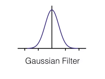
Gaussian Processes - Covariance function Squared exponential (or Gaussian) covariance function: Perry Groot , Markus Peters � � N − 1 Tom Heskes, � n ) 2 k ( x , x ′ ) = exp ( x n − x ′ Wolgang 2 θ 2 Ketter n = 1 Introduction where θ is a length-scale parameter denoting how quickly Background the functions are to vary. GPs Laplace Approximation Kronecker product length−scale 0.5 length−scale 2 2.5 2.5 MAP estimation 2 2 Model 1.5 1.5 Selection 1 1 Experiment 0.5 0.5 0 0 −0.5 −0.5 −1 −1 −1.5 −1.5 0 2 4 6 8 10 0 2 4 6 8 10

Gaussian Processes - 1D demo Perry Groot , 10 10 Markus Peters Tom Heskes, 5 5 Wolgang Ketter 0 0 Introduction −5 −5 Background GPs −10 −10 Laplace Approximation 0 2 4 6 8 10 0 2 4 6 8 10 Kronecker product MAP estimation 10 10 Model Selection 5 5 Experiment 0 0 −5 −5 −10 −10 0 2 4 6 8 10 0 2 4 6 8 10

Laplace Approximation Perry Groot , Markus Peters Tom Heskes, Wolgang Ketter For Gaussian process models with non-gaussian likelihood models we need approximations. Introduction Background GPs Laplace: approximate true posterior p ( f | X , y ) with a Laplace Approximation Gaussian q ( f ) centered on the mode of the posterior: Kronecker product MAP estimation f , ( K − 1 + W ) − 1 ) q ( f ) = N ( f | ˆ (1) Model Selection with ˆ f = arg max f p ( f | X , y , θ ) and W = −∇∇ f log p ( y | f ) | f =ˆ f . Experiment

Kronecker product Assumptions Perry Groot , Tensor product kernel function: Markus Peters Tom Heskes, k ( x i , x j ) = � D d = 1 k d ( x d i , x d j ) . Wolgang Ketter data on multi-dimensional grid Introduction Background This results in a kernel matrix that decomposes into a GPs Laplace Approximation Kronecker product of matrices of lower dimensions. Kronecker product MAP estimation K = K 1 ⊗ · · · ⊗ K D Model Selection where Experiment   a 11 B · · · a 1 n B . . ...  . .  A ⊗ B = . .   · · · a m 1 B a mn B

Kronecker product Perry Groot , Markus Peters The Kronecker product has a convenient algebra Tom Heskes, Wolgang Ketter ( A ⊗ B ) vec ( X ) = vec ( BXA T ) Introduction AB ⊗ CD = ( A ⊗ C )( B ⊗ D ) Background GPs ( A ⊗ B ) − 1 = A − 1 ⊗ B − 1 Laplace Approximation Kronecker product MAP estimation Operation Standard Kronecker Model Selection O ( � D O ( N 2 ) d = 1 N 2 d ) Storage Experiment O ( N ( � D O ( N 2 ) Matrix vector product d = 1 N d )) O ( � D O ( N 3 ) d = 1 N 3 Cholesky / SVD d )

MAP estimation Perry Groot , Markus Peters Tom Heskes, Let b = Wf + ∇ log p ( y | f ) . We need Wolgang Ketter f new = ( K − 1 + W ) − 1 b Introduction 1 1 1 1 Background 2 ) − 1 W 2 ( I + W 2 KW 2 K ) b = K ( I − W GPs � �� � Laplace Approximation v Kronecker product MAP Repeat until convergence: estimation 1 1 1 Model 2 KW 2 ) v = W 2 Kb iteratively solve ( I + W Selection 1 Experiment 2 v a = b − W f = Ka

Marginal Likelihood Perry Groot , Markus Peters Tom Heskes, Wolgang Ketter learn the value of θ , which can be done by minimizing the Introduction negative marginal likelihood Background GPs Laplace Approximation − log p ( y | X , θ ) ≈ 1 f ) + 1 T K − 1 ˆ ˆ f − log p ( y | ˆ Kronecker product f 2 log | B | 2 MAP estimation with B = I + KW . Model Selection Experiment

Reduced-rank approximation Perry Groot , We use a reduced-rank approximation: Markus Peters Tom Heskes, Wolgang K ≈ QSQ T + Λ 1 Ketter Introduction with Background GPs Laplace D Approximation � Kronecker product Q = Q d , N × R matrix MAP estimation d = 1 Model D � Selection S = S d , R × R matrix Experiment d = 1 Λ 1 = diag ( diag ( K ) − diag ( QSQ T ))

Evaluating Marginal Likelihood Perry Groot , Markus Peters Tom Heskes, Wolgang Ketter 1 1 Introduction 2 KW 2 | | B | = | I + W Background 1 1 1 1 GPs 2 QSQ T W 2 + W 2 | ≈ | I + W 2 Λ 1 W Laplace Approximation Kronecker product 1 1 2 QSQ T W 2 | = | Λ 2 + W MAP estimation = | Λ 2 || S || S − 1 + Q T W 1 1 2 Λ − 1 2 Q | 2 W Model Selection = | Λ 2 || S || S − 1 + Q T Λ 3 Q | Experiment

Gradients Perry Groot , Markus Peters Need the gradients wrt θ of Tom Heskes, Wolgang Ketter − log p ( y | X , θ ) ≈ 1 f ) + 1 T K − 1 ˆ ˆ f − log p ( y | ˆ 2 log | B | f Introduction 2 Background GPs which is given by Laplace Approximation Kronecker product � ∂ log q ( y | X , θ ) = ∂ log q ( y | X , θ ) � MAP � estimation ∂θ j ∂θ j � explicit Model Selection N ∂ ˆ ∂ log q ( y | X , θ ) f i � Experiment + ∂ ˆ ∂θ j f i i = 1

Explicit Derivatives – Kernel Hyperparameters Perry Groot , Markus Peters Tom Heskes, Wolgang Ketter Given by Introduction � Background ∂ log q ( y | X , θ ) � = 1 T K − 1 ∂ K ˆ K − 1 ˆ � GPs f f � ∂θ c ∂θ c Laplace 2 � Approximation j j explicit Kronecker product � � MAP − 1 ( W − 1 + K ) − 1 ∂ K estimation . 2 tr ∂θ c Model j Selection Experiment

Explicit Derivatives – Kernel Hyperparameters Perry Groot , Markus Peters Tom Heskes, Wolgang Ketter ( W − 1 + K ) − 1 Introduction 1 1 1 1 Background 2 ) − 1 W 2 ( I + W 2 KW = W 2 GPs Laplace 1 1 1 1 1 1 Approximation 2 QSQ T W 2 ) − 1 W 2 ( I + W 2 + W ≈ W 2 Λ W 2 Kronecker product MAP 1 1 1 1 2 QSQ T W 2 ) − 1 W 2 ( Λ 2 + W = W estimation 2 Model 2 Q ( S − 1 + Q T Λ − 1 1 1 1 2 ( Λ − 1 − Λ − 1 3 Q ) − 1 Q T W 2 Λ − 1 Selection = W 2 W 2 ) W 2 Experiment = Λ 3 − Λ 3 Q ( S − 1 + Q T Λ 3 Q ) − 1 Q T Λ 3

Explicit Derivatives – Kernel Hyperparameters Perry Groot , Markus Peters Tom Heskes, Wolgang Ketter �� � � − 1 ∂ K W − 1 + K tr Introduction ∂θ c j Background � � � � GPs ∂ K � � − 1 ∂ K Laplace S − 1 + Q T Λ 3 Q Q T Λ 3 Approximation = tr − tr Λ 3 Q Λ 3 Kronecker product ∂θ c ∂θ c j j MAP estimation � � � � ∂ K ∂ K Model V T = tr Λ 3 − tr V 1 Selection 1 ∂θ c ∂θ c j j Experiment � ( S − 1 + Q T Λ 3 Q ) − 1 � with V 1 = Λ 3 Q chol .

Remaining Gradients Perry Groot , Markus Peters Tom Heskes, Wolgang Ketter Similar arguments for computing the remaining gradients Introduction Background Linear Algebra Shortcuts GPs Laplace Approximation tr ( ABC ) = tr ( BCA ) Kronecker product MAP tr ( AB T ) = S UM R OWS ( A ◦ B ) estimation diag ( ABC T ) = ( A ◦ C ) · diag ( B ) when B is diagonal Model Selection Experiment

Experiment Artificial classification data generated on X = [ 0 , 1 ] 2 with Perry Groot , Markus Peters Tom Heskes, various grid sizes. Wolgang Ketter Introduction 1100 Standard Kronecker 1000 Background GPs 900 Laplace 800 Approximation Kronecker product 700 seconds MAP 600 estimation 500 Model 400 Selection 300 Experiment 200 100 1000 2000 3000 4000 5000 6000 N