Fast High-Dimensional Feature Matching for Object Recognition - PowerPoint PPT Presentation
Fast High-Dimensional Feature Matching for Object Recognition David Lowe Computer Science Department University of British Columbia Finding the panoramas Finding the panoramas Finding the panoramas Location recognition The Problem
Fast High-Dimensional Feature Matching for Object Recognition David Lowe Computer Science Department University of British Columbia
Finding the panoramas
Finding the panoramas
Finding the panoramas
Location recognition
The Problem � Match high-dimensional features to a database of features from previous images � Dominant cost for many recognition problems � Typical feature dimensionality: 128 dimensions � Typical number of features: 1000 to 10 million � Time requirements: Match 1000 features in 0.1 to 0.01 seconds � Applications � Location recognition for a mobile vehicle or cell phone � Object recognition for database of 10,000 images � Identify all matches among 100 digital camera photos
Invariant Local Features � Image content is transformed into local feature coordinates that are invariant to translation, rotation, scale, and other imaging parameters SIFT Features
Build Scale-Space Pyramid � All scales must be examined to identify scale-invariant features � An efficient function is to compute the Difference of Gaussian (DOG) pyramid (Burt & Adelson, 1983) Resample l p m e R r u l B s a e s a B l u e l p m r e R u a c b t r t t S a c r t b u S Blur Subtract
Key point localization � Detect maxima and minima of difference-of- Gaussian in scale space e e l p m s a R r u l B S u b t r a c t
Select dominant orientation � Create histogram of local gradient directions computed at selected scale � Assign canonical orientation at peak of smoothed histogram 2 π 0
SIFT vector formation � Thresholded image gradients are sampled over 16x16 array of locations in scale space � Create array of orientation histograms � 8 orientations x 4x4 histogram array = 128 dimensions
Distinctiveness of features � Vary size of database of features, with 30 degree affine change, 2% image noise � Measure % correct for single nearest neighbor match
Approximate k-d tree matching Arya, Mount, et al., “An optimal algorithm for approximate � nearest neighbor searching,” Journal of the ACM, (1998). � Original idea from 1993 Best-bin-first algorithm (Beis & Lowe, 1997) � � Uses constant time cutoff rather than distance cutoff Key idea: � Search k-d tree bins in order of distance from query � Requires use of a priority queue
Results for uniform distribution Compares original � k-d tree (restricted search) with BBF priority search order (100,000 points with cutoff after 200 checks) Results: Close neighbor � found almost all the time Non-exponential � increase with dimension!
Probability of correct match � Compare distance of nearest neighbor to second nearest neighbor (from different object) � Threshold of 0.8 provides excellent separation
Fraction of nearest neighbors found 100,000 uniform � points in 12 dimensions. Results: Closest neighbor � found almost all the time Continuing � improvement with number of neighbors examined
Practical approach that we use � Use best bin search order of k-d tree with a priority queue � Cut off search after amount of time determined so that nearest-neighbor computation does not dominate � Typically cut off after checking 100 leaves � Results: � Speedup over linear search by factor of 5,000 for database of 1 million features � Find 90-95% of useful matches � No improvements from ball trees, LSH,… � Wanted: Ideas to find those last 10% of features
Sony Aibo SIFT usage: Recognize charging station Communicate with visual cards
Example application: Lane Hawk � Recognize any of 10,000 images of products in a grocery store � Monitor all carts passing at rate of 3 images/sec � Now available
Recognition in large databases
Conclusions � Approximate NN search with k-d tree using priority search order works amazingly well! � Many people still refuse to believe this � Constant time search cutoff works well in practice � I have yet to find a better method in practice
Recommend
More recommend
Explore More Topics
Stay informed with curated content and fresh updates.
