Optimal Estimation of Matching Constraints 1 Motivation & - PowerPoint PPT Presentation

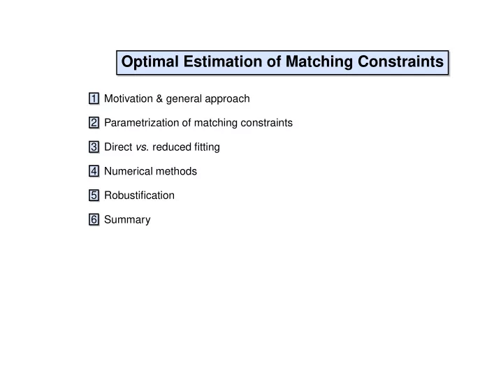
Optimal Estimation of Matching Constraints 1 Motivation & general approach 2 Parametrization of matching constraints 3 Direct vs. reduced fitting 4 Numerical methods 5 Robustification 6 Summary

Why Study Matching Constraint Estimation? : : : 1 They are practically useful , both for correspondence and reconstruction 2 They are algebraically complicated , so the best algorithm is not obvious — a good testing ground for new ideas 3 There are many variants ) Try a systematic approach rather than an ad hoc case-by-case one — different constraint & feature types, camera models — special forms for degenerate motions and scene geometries

� For practical reliability, it is essential to use an appropriate model � Model selection methods fit several models, choose the best Model selection ) many fits are to inappropriate models (strongly biased, degenerate) ) the fitting algorithm must be efficient and reliable, even in difficult cases

Questions to Study 1 How much difference does an accurate statistical error model make ? 2 Which types of constraint parametrization are the most reliable ? 3 Which numerical method offers the best stability/speed/simplicity ? The answers are most interesting for nearly degenerate cases, as these are the most difficult to handle reliably.

� Separate modules for Design of Library 1. Modular Architecture 1 matching geometry type & parametrization 2 feature type, parametrization & error model 3 linear algebra implementation 4 loop controller (step damping, convergence tests)

de e ( x ) dx > 2 Stable Gauss-Newton Approach d ( j e j ) de de de > = e ; dx dx dx dx 1 Work with residual error vectors and Jacobians � e.g. simplest residual is e = x � x 2 > d e e 2 dx — not gradient and Hessian of squared error + Cholesky for observations x 2 Discard 2nd derivatives, e.g. 3 For stability use QR decomposition, not normal equations Advantages of Gauss-Newton + Simple to use — no 2nd derivatives required + Stable linear least squares methods can be used for step prediction – Convergence may be slow if problem has both large residual and strong nonlinearity — but in vision, residuals are usually small

� The underlying geometry of matching constraints is parametrized by nontrivial Parametrization of Matching Geometry � the variety of all homographic mappings between algebraic varieties — there are no single, simple, minimal parametrizations — e.g. epipolar geometry line pencils in two images There are (at least) three ways to parametrize varieties: 1 Implicit constraints on some higher dimensional space 2 Overlapping local coordinate patches 3 Redundant parametrizations with internal gauge freedoms

Constrained Parametrizations 1 Embed the variety in a larger ( e.g. linear, tensor) space 2 Find consistency conditions that characterize the embedding Matching Tensors are the most familiar embeddings � Other useful embeddings of matching geometry may exist : : : — coefficients of multilinear feature matching relations � Typical consistency conditions: — e.g. the fundamental matrix F det ( F ) = 0 3 d det ( G � x ) = 0 : : : 3 d x — fundamental matrix: — trifocal tensor: plus others

Advantages of Constrained Parametrizations + Very natural when matching geometry is derived from image data + “Linear methods” give (inconsistent!) initial estimates – Reconstruction problem — how to go from tensor to other properties of matching geometry – The consistency conditions rapidly become complicated and non-obvious > codimension — Demazure for essential matrix — Faugeras-Papadopoulo for the trifocal tensor – Constraint redundancy is common: #generators

� e.g. describe some components of a matching tensor as nonlinear functions Local Coordinates / Minimal Parametrizations � � a b c Express the geometry in terms of a minimal set of independent parameters d e f � c.f. Z. Zhang’s F = det ( F ) = 0 ua + v d ub + v e uc + v f of the others (or of some other parameters) guarantees

Advantages of Minimal Parametrizations + Simple unconstrained optimization methods can be used – They are usually highly anisotropic — they don’t respect symmetries of the underlying geometry so they are messy to implement, and hard to optimize over – They are usually only valid locally — many coordinate patches may be needed to cover the variety, plus code to manage inter-patch transitions – They must usually be found by algebraic elimination using the constraints — numerically ill-conditioned, and rapidly becomes intractable It is usually preferable to eliminate variables numerically using the constraint Jacobians — i.e. constrained optimization

Redundant Parametrizations / Gauge Freedom In many geometric problems, the simplest approach requires an arbitrary choice of coordinate system ! � F Common examples: 1 3D coordinate frames in reconstruction, projection-based matching constraint parametrizations ' [ e ] ! H + e a � H 2 Homogeneous-projective scale factors F � H � � H � � e � 0 0 0 0 0 0 0 00 > ' e � H � H � e ! + 0 0 0 0 00 3 Homographic parametrizations of epipolar and trifocal geometry F with freedom H for any a G a with freedom H H e

Gauge Freedoms � Gauge just means (internal) coordinate system � There is an associated symmetry group and its representations Gauge Freedoms are internal symmetries associated with a free choice of internal “coordinates” � Expressions derived in gauged coordinates reflect the symmetries � A familiar example: ordinary 3D Cartesian coordinates — the gauge group is the rigid motions — the gauged representations are Cartesian tensors

Advantages of Gauged Parametrizations + Very natural when the matching geometry is derived from the 3D one + Close to the geometry, so it is easy to derive further properties from them + Numerically much stabler than minimal parametrizations + One coordinate system covers the whole variety – Symmetry implies rank degeneracy — special numerical methods are needed – They may be slow as there are additional, redundant variables

Handling Gauge Freedom Numerically � If left undamped, large gauge fluctuations can destabilize the system Gauge motions don’t change the residual, so there is nothing to say what they should be � Control fluctuations by � C.f. ‘Free Bundle’ methods in photogrammetry — e.g. Hessians are exactly rank deficient in the gauge directions gauge fixing conditions or free gauge methods

� Remove the degeneracy by adding artificial constraints P = ( I j 0 ) , e � H = 0 1 3 � 3 1. Gauge Fixing Conditions � Constrained optimization is (usually) needed � Poorly chosen constraints can increase ill-conditioning — e.g. Hartley’s gauges 2. ‘Free Gauge’ Methods 1 Leave the gauge “free to drift” — but take care not to push it too hard ! — rank deficient least squares methods (basic or min. norm solutions) — Householder reduction projects motion orthogonally to gauge directions 2 Monitor the gauge and reset it “by hand” as necessary ( e.g. each iteration)

> F x = 0 Constrained Optimization det ( F ) = 0 2 Constraints arise from � H = 0 , k F k = 1 1 Matching relations on features, e.g. x 2 Consistency conditions on matching tensors, e.g. 3 Gauge fixing conditions , e.g. e

Approaches to Constrained Optimization 1 Eliminate variables numerically using constraint Jacobian : : : 2 Introduce Lagrange multipliers and solve for these too — for dense systems, 2 is simpler but 1 is usually faster and stabler � The linear algebra gets complicated, especially for sparse problems — each has many variants: linear algebra method, operation ordering, � A lack of efficient, reliable search control heuristics Difficulties � Constraint redundancy

> codimension 8 < = codimension on the variety Constraint Redundancy : > codimension away from it Many algebraic varieties have #generators � Examples rank 0 00 The constraint Jacobian has ] ( G ] [ x � x ) [ x � � has rank 3 for valid trifocal rank 3 d det ( G � x ) has rank 8 for valid 3 d x 1 the trifocal point constraint tensors, 4 otherwise � It seems difficult to handle such localized redundancies numerically 2 the trifocal consistency constraint � Currently, I assume known codimension r , project out the strongest r tensors, 10 otherwise constraints and enforce only these

Abstract Geometric Fitting Problem x i u 1. Model-Feature Constraints There are 1 Unknown true underlying ‘features’ c ( x ; u ) = 0 i i 2 An unknown true underlying ‘model’ 3 Exactly satisfied model-feature consistency constraints � E.g. for epipolar geometry 0 ( x ; x ) i i u is the fundamental matrix F > 0 = 0 i F x i — a ‘feature’ is a pair of corresponding points — the ‘model’ — the ‘model-feature constraint’ is the epipolar constraint x

2. Error Model � ( x ) = � ( x j observations i ) i i i i 1 There is an additive posterior statistical error metric linking the underlying features to observations and other prior information � prior ( u ) 0 � For epipolar geometry, given observed points ( x ; x ) , we could take — e.g. (robustified, bias corrected) posterior log likelihood � � 0 2 0 0 2 2 There may also be a model-space prior � ( x ; x ) = � k x � x k + k x � x k � ( � ) is some robustifier where