Fast classification using sparsely active spiking networks Hesham - PowerPoint PPT Presentation
Fast classification using sparsely active spiking networks Hesham Mostafa Institute of neural computation, UCSD Artificial networks vs. spiking networks backpropagation output layer ...... ...... Multi-layer networks are extremely hidden
Fast classification using sparsely active spiking networks Hesham Mostafa Institute of neural computation, UCSD
Artificial networks vs. spiking networks backpropagation output layer ...... ...... Multi-layer networks are extremely hidden layer 2 powerful function approximators. hidden layer 1 Backpropagation is the most effective method we know of to input layer solve the credit assignment problem in deep artificial networks ??? output layer ...... How do we solve the credit assignment hidden layer 2 problem in multi-layer spiking networks? hidden layer 1 input layer
Neural codes and gradient descent Rate coding: Temporal coding ● Spike counts/rates are discrete quantities ● Spike times are analog quantities ● Gradient is zero almost everywhere ● Gradient of output spike time w.r.t input ● Only indirect or approximate gradient spike times is well-defined and non-zero ● Direct gradient descent training possible descent training possible input output input output 3 t1 t1 5 4 tOut t2 t2 2 tOut t3 t3
The neuron model 1.2 1.0 0.8 Vmem Non-leaky integrate and fire neuron 0.6 dVmem ( t ) 0.4 = Isyn ( t ) (firing threshold is 1) dt 0.2 0.0 0.0 0.5 1.0 1.5 2.0 2.5 3.0 3.5 4.0 1.0 Exponentially decaying synaptic current 0.8 Isyn ( t )= ∑ w i exp (−( t − t i ))Θ( t − t i ) Isyn 0.6 i Θ( t − t i ) : Step function 0.4 0.2 0.0 0.0 0.5 1.0 1.5 2.0 2.5 3.0 3.5 4.0 time
The neuron's transfer function tout 1.2 1.0 0.8 Vmem 0.6 0.4 0.2 0.0 0.0 0.5 1.0 1.5 2.0 2.5 3.0 3.5 4.0 t1 t2 t3 t4 1.0 0.8 0.6 Isyn w3 0.4 w4 w2 0.2 w1 0.0 0.0 0.5 1.0 1.5 2.0 2.5 3.0 3.5 4.0 time
The neuron's transfer function In general: tout 1.2 1.0 0.8 Vmem 0.6 0.4 Where C is the causal set of input 0.2 spikes (input spikes that arrive before output spike) 0.0 0.0 0.5 1.0 1.5 2.0 2.5 3.0 3.5 4.0 t1 t2 t3 t4 1.0 0.8 0.6 Isyn w3 0.4 w4 w2 0.2 w1 0.0 0.0 0.5 1.0 1.5 2.0 2.5 3.0 3.5 4.0 time
The neuron's transfer function In general: tout 1.2 1.0 0.8 Vmem 0.6 0.4 Where C is the causal set of input 0.2 spikes (input spikes that arrive before output spike) 0.0 0.0 0.5 1.0 1.5 2.0 2.5 3.0 3.5 4.0 t1 t2 t3 t4 1.0 Time of the L th output spike: 0.8 0.6 Isyn w3 0.4 w4 w2 0.2 w1 0.0 0.0 0.5 1.0 1.5 2.0 2.5 3.0 3.5 4.0 time
Change of variables The neuron's transfer function then becomes piece-wise linear in the inputs (but not the weights):
Where is the non-linearity? Non-linearity arises due to the input dependence of the causal set of input spikes The piecewise linear input-output relation is reminiscent of Rectified Linear Units (ReLU) networks ln(z out ) ln(z out ) 1.2 1.2 z out = w 1 z 1 +w 2 z 2 +w 3 z 3 z out = w 1 z 1 +w 2 z 2 +w 3 z 3 +w 4 z 4 1.0 w 1 +w 2 +w 3 −1 1.0 w 1 +w 2 +w 3 +w 4 −1 0.8 0.8 vmem vmem 0.6 0.6 0.4 0.4 0.2 0.2 0.0 0.0 0.0 0.5 1.0 1.5 2.0 2.5 3.0 3.5 4.0 0.0 0.5 1.0 1.5 2.0 2.5 3.0 3.5 4.0 ln(z 1 ) ln(z 2 )ln(z 3 ) ln(z 4 ) ln(z 1 ) ln(z 2 ) ln(z 3 )ln(z 4 ) synaptic current synaptic current 1.0 1.0 0.8 0.8 0.6 0.6 0.4 0.4 0.2 0.2 0.0 0.0 0.0 0.5 1.0 1.5 2.0 2.5 3.0 3.5 4.0 0.0 0.5 1.0 1.5 2.0 2.5 3.0 3.5 4.0 time time
What is the form of computation implemented by the temporal dynamics? ln(z out ) 1.2 z out = w 1 z 1 +w 2 z 2 +w 3 z 3 1.0 w 1 +w 2 +w 3 −1 0.8 vmem 0.6 0.4 0.2 .... 0.0 0.0 0.5 1.0 1.5 2.0 2.5 3.0 3.5 4.0 ln(z 1 ) ln(z 2 )ln(z 3 ) ln(z 4 ) synaptic current 1.0 0.8 0.6 0.4 0.2 0.0 ● To compute zout: 0.0 0.5 1.0 1.5 2.0 2.5 3.0 3.5 4.0 time ● Sort {z1,z2,..,zn} ● Find the causal set, C, by progressively considering more early spikes ● Calculate Can not be reduced to the conventional ANN neuron: z out = f ( ∑ w i z i ) i
Backpropagation To use backpropagation to train a multi-layer network, we need the derivatives of the neuron's output w.r.t: Weights Inputs Time of first spike encodes neuron’s value. Each neuron is allowed to spike only once in response to an input pattern: ● Forces sparse activity. Training has to make maximum use of each spike ● Allows quick classification response
Classification Tasks ● We can relate the time of any spike differentiably to the times of all spikes that caused it ● We can impose any differentiable cost function on the spike times of the output layer and use backpropagation to minimize cost across training set ● In a classification setting, use a loss function that encourages the output neuron representing the correct class to spike first ● Since we have an analytical input-output relation for each neuron, training can be done using conventional machine learning packages (Theano/Tensorflow)
MNIST task ● Pixel values were binarized. ● High intensity pixels spike early ● Low intensity pixels spike late
Classification is extremely rapid ● A decision is made when the first output neuron spikes ● A decision is made after only 25 spikes (on average) from the hidden layer in the 768-800-10 network, i.e, only 3% of the hidden layer neurons contribute to each classification decision
FPGA prototype 1400 1400 1200 1200 1000 1000 Mean : 30 800 800 Mean : 167 Count Count Median : 29 Median : 162 600 600 400 400 200 200 0 0 0 20 40 60 80 100 120 140 160 180 0 100 200 300 400 500 600 Number of hidden layer spikes before output spike Timesteps to classifjcation ● 97% test set classification accuracy on MNIST in a 784-600-10 network (8-bit weights) ● Average number of spikes until classification: 139 ● Only 13% of input to hidden weights are looked up ● Only 5% of hidden to output weights are looked up
Acknowledgements Giacomo Indiveri Tobi Delbruck Institute of neuroinformatics Gert Cauwenberghs Sadique Sheik Bruno Pedroi
Approximate learning correct label Output N7 N8 N9 layer - - + + + Hidden layer N4 N5 N6 - + - + Input layer N1 N2 N3 ● Update Hidden→Output weights to encourage the right neuron to spike first ● Only update weights that actually contributed to output timings
Approximate learning correct label Output N7 N8 N9 layer - - + + + -1 } +1 } Hidden +1 -1 -(-1) layer N4 N5 N6 - + - + Input layer N1 N2 N3 ● Backpropagate time deltas using only the sign of the weights ● The final time delta at a hidden layer neuron can be obtained using 2 parallel popcount operations (count 1s in a bit vector) and a comparison.
Recommend
More recommend
Explore More Topics
Stay informed with curated content and fresh updates.
