Exploring the Limits of Classification Accuracy Carolyn Kim 1 Lester - PowerPoint PPT Presentation
Exploring the Limits of Classification Accuracy Carolyn Kim 1 Lester Mackey 2 1 Computer Science Department, Stanford University 2 Statistics Department, Stanford University December 7, 2015 Carolyn Kim , Lester Mackey (Stanford) Exploring the
Exploring the Limits of Classification Accuracy Carolyn Kim 1 Lester Mackey 2 1 Computer Science Department, Stanford University 2 Statistics Department, Stanford University December 7, 2015 Carolyn Kim , Lester Mackey (Stanford) Exploring the Limits of Classification Accuracy December 7, 2015 1 / 16
Classification Setup: random variable ( X , Y ), where X describes the observations, and Y describes the class label In our case, X takes values in R d (jet images), and Y takes values in ± 1 (“signal” W-jets or “background” QCD-jets). We can construct a classifier: g : R d → {± 1 } , with loss L ( g ) := P { g ( X ) � = Y } We want the optimal classifier ( Bayes Classifier ) g ∗ = argmin P { g ( X ) � = Y } g : R d →{± 1 } L ∗ := L ( g ∗ ) g ∗ is the classifier that outputs 1 if P { 1 | x } > P {− 1 | x } Carolyn Kim , Lester Mackey (Stanford) Exploring the Limits of Classification Accuracy December 7, 2015 2 / 16
k-Nearest Neighbors The k-nearest neighbor classifier g k , n given n samples ( X 1 , Y 1 ) , . . . , ( X n , Y n ) with weights w 1 , . . . , w n is � � 1 w i > w i X i ∈{ k − nearest neighbors ( x ) } X i ∈{ k − nearest neighbors ( x ) } g k , n ( x ) = Yi =1 Yi = − 1 − 1 otherwise Theorem (Universal Consistency of k-Nearest Neighbors, Deyvroye and Gyorfi, 1985, Zhao (1987)) For any distribution of ( X , Y ) , as k → ∞ , k / n → 0 , n → ∞ , i.i.d. samples, then L ( g k , n ) → L ∗ . Theorem (Devroye, 1981) � For k ≥ 3 and odd, lim n →∞ L ( g 1 , n ) ≤ L ∗ (1 + 2 k ) . Carolyn Kim , Lester Mackey (Stanford) Exploring the Limits of Classification Accuracy December 7, 2015 3 / 16
Experimental setup Generate data: simulated signal and background events with p t ∈ [200 , 400] GeV; each event is defined by a weight and 20-40 particles defined by ( φ , η , energy). Bin data, resulting in a jet image, a vector in R d . Optionally, whiten the data so the training covariance matrix is the identity. Compute the distances to the k -th nearest signal and background neighbors (this is enough information to do 2 k − 1-nearest neighbor) in the “distance training set” ( 900K or 10M in size). In practice, this requires a lot of computational power! create a rejection versus efficiency curve Carolyn Kim , Lester Mackey (Stanford) Exploring the Limits of Classification Accuracy December 7, 2015 4 / 16
Step 1: Binning Multiple possible binning strategies: equal size binning or equal weight (event weight only vs. event weight * energy bin bounds, energy only bin values vs energy density bin values) Figure 1: Sample bin bounds for an equal weighting scheme Carolyn Kim , Lester Mackey (Stanford) Exploring the Limits of Classification Accuracy December 7, 2015 5 / 16
Mean heatmap of one binning strategy Carolyn Kim , Lester Mackey (Stanford) Exploring the Limits of Classification Accuracy December 7, 2015 6 / 16
Plotting rejection versus efficiency curve x -axis is signal efficiency (proportion of signal classified as signal) y -axis is 1 − background efficiency The 1-D discriminant is the ratio between the probability densities of distances to the k -th nearest signal and background neighbor. (2D-likelihood without taking the ratio has empirically not been better.) use one set of distances as a “curve training” set to estimate the densities, and another set of distances as the “curve testing” set to plot the curve Carolyn Kim , Lester Mackey (Stanford) Exploring the Limits of Classification Accuracy December 7, 2015 7 / 16
curve training, testing: 100K; distance training: 900K Carolyn Kim , Lester Mackey (Stanford) Exploring the Limits of Classification Accuracy December 7, 2015 8 / 16
curve training, testing: 100K; distance training: 900K Carolyn Kim , Lester Mackey (Stanford) Exploring the Limits of Classification Accuracy December 7, 2015 9 / 16
curve training, testing: 100K; distance training: 900K Carolyn Kim , Lester Mackey (Stanford) Exploring the Limits of Classification Accuracy December 7, 2015 10 / 16
curve training, testing: 1M; distance training: 10M Carolyn Kim , Lester Mackey (Stanford) Exploring the Limits of Classification Accuracy December 7, 2015 11 / 16
curve training, testing: 1M; distance training: 10M How well are we doing? Unfortunately, worse than mass... Carolyn Kim , Lester Mackey (Stanford) Exploring the Limits of Classification Accuracy December 7, 2015 12 / 16
Kernels A kernel function K : R d → R intuitively creates “bumps” around 0 (e.g. Gaussian kernel K ( x ) = e −� x � 2 ). We can estimate the probability density function by summing up kernel functions centered at the data points: P ( y j | x ) ∝ � Y i = y j w i K ( x − X i ) ∼ Credit: http://en.wikipedia.org Carolyn Kim , Lester Mackey (Stanford) Exploring the Limits of Classification Accuracy December 7, 2015 13 / 16
The kernel classifier g K , n for a kernel function K given n samples ( X 1 , Y 1 ) , . . . , ( X n , Y n ) with weights w 1 , . . . , w n is w i K ( x − X i w i K ( x − X i 1 � ) > � ) h h g K , n ( x ) = Y i =1 Y i = − 1 − 1 otherwise Theorem (Devroye and Kryzyzak, 1989) For any distribution of ( X , Y ) , if h → 0 and nh d → ∞ as n → ∞ , i.i.d. samples, then L ( g Gaussian , n ) → L ∗ . This classifier can converge faster than the k-NN estimator if the conditional densities are smooth. Carolyn Kim , Lester Mackey (Stanford) Exploring the Limits of Classification Accuracy December 7, 2015 14 / 16
Random Fourier Feature Kernel Density Estimation Randomized algorithm to approximate the Gaussian kernel, which makes it more efficient (at least a 10x speedup.) Carolyn Kim , Lester Mackey (Stanford) Exploring the Limits of Classification Accuracy December 7, 2015 15 / 16
Next Steps Use FLANN, a library for fast approximate nearest neighbors. Scale to higher dimensions: currently it takes 10 hours to run 81-dimensional data; use more data! Tune random Fourier Feature parameters Other strategies: e.g. use independent component analysis Carolyn Kim , Lester Mackey (Stanford) Exploring the Limits of Classification Accuracy December 7, 2015 16 / 16
Recommend
More recommend
Explore More Topics
Stay informed with curated content and fresh updates.


