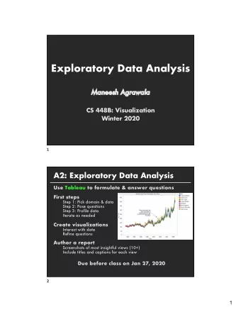
Exploratory data analysis R F OR S AS US ERS Melinda Higgins, PhD - PowerPoint PPT Presentation

Exploratory data analysis R F OR S AS US ERS Melinda Higgins, PhD Research Professor/Senior Biostatistician Emory University

Summary statistics R FOR SAS USERS

R FOR SAS USERS

R FOR SAS USERS

R FOR SAS USERS

Summary statistics # Summary statistics of weight, height, bmi of daviskeep daviskeep %>% select(weight, height, bmi) %>% summary() weight height bmi Min. : 39.0 Min. :148.0 Min. :15.82 1st Qu.: 55.0 1st Qu.:164.0 1st Qu.:20.22 Median : 63.0 Median :170.0 Median :21.80 Mean : 65.3 Mean :170.6 Mean :22.26 3rd Qu.: 73.5 3rd Qu.:177.5 3rd Qu.:23.94 Max. :119.0 Max. :197.0 Max. :36.73 R FOR SAS USERS

Descriptive statistics with Hmisc # Load Hmisc, run describe() for sex and bmi library(Hmisc) ----------------------------------------------------- daviskeep %>% bmi select(sex, bmi) %>% n missing distinct Info Mean Gmd Hmisc::describe() 199 0 176 1 22.26 3.303 .05 .10 .25 .50 .75 .90 18.05 18.84 20.22 21.80 23.94 26.30 2 Variables 199 Observations .95 ----------------------------------------------------- 27.25 sex lowest : 15.82214 16.93703 17.09928 17.43285 17.50639 n missing distinct highest: 29.73704 29.80278 30.09496 30.15916 36.72840 199 0 2 Value F M Frequency 111 88 Proportion 0.558 0.442 R FOR SAS USERS

Descriptive statistics with psych # Load psych package, run psych:: describe() for weight, height, bmi library(psych) daviskeep %>% select(weight, height, bmi) %>% psych::describe() Result vars n mean sd median trimmed mad min max range skew kurtosis se weight 1 199 65.30 13.34 63.0 64.12 11.86 39.00 119.00 80.00 0.91 0.84 0.95 height 2 199 170.59 8.95 170.0 170.40 10.38 148.00 197.00 49.00 0.21 -0.38 0.63 bmi 3 199 22.26 3.01 21.8 22.08 2.55 15.82 36.73 20.91 0.91 1.91 0.21 R FOR SAS USERS

Speci�c statistic summaries R FOR SAS USERS

R FOR SAS USERS

Speci�c statistic summaries - one variable # For height, get n, median, 5th, 95th quartiles, min, max daviskeep %>% summarise(nht = n(), medianht = median(height), pt05 = quantile(height, probs = 0.05), pt95 = quantile(height, probs = 0.95), minht = min(height), maxht = max(height)) Result nht medianht pt05 pt95 minht maxht 1 199 170 157 185 148 197 R FOR SAS USERS

R FOR SAS USERS

Speci�c statistic summaries - multiple variables # For weight, height and bmi, get mean, standard deviation daviskeep %>% select(weight, height, bmi) %>% summarise_all(funs(mean, sd)) Result weight_mean height_mean bmi_mean weight_sd height_sd bmi_sd 1 65.29648 170.5879 22.25761 13.34346 8.948848 3.009239 R FOR SAS USERS

R FOR SAS USERS

Summary statistics - by group # Get mean and sd for weight, height and bmi by sex group daviskeep %>% group_by(sex) %>% select(sex, weight, height, bmi) %>% summarise_all(funs(mean, sd)) # A tibble: 2 x 7 sex weight_mean height_mean bmi_mean weight_sd height_sd bmi_sd <fct> <dbl> <dbl> <dbl> <dbl> <dbl> <dbl> 1 F 56.9 165. 21.0 6.89 5.68 2.18 2 M 75.9 178. 23.9 11.9 6.44 3.12 R FOR SAS USERS

Let's summarise abalones! R F OR S AS US ERS

Correlations and t- tests R F OR S AS US ERS Melinda Higgins, PhD Research Professor/Senior Biostatistician Emory University

Correlations compare SAS and R R FOR SAS USERS

R FOR SAS USERS

Correlations with psych package # Correlations with psych::corr.test() Call:psych::corr.test(x = .) daviskeep %>% Correlation matrix select(bmi, weight, height) %>% bmi weight height psych::corr.test() bmi 1.00 0.88 0.38 weight 0.88 1.00 0.77 height 0.38 0.77 1.00 Sample Size [1] 199 Probability values (Entries above the diagonal are adjusted for multiple tests.) bmi weight height bmi 0 0 0 weight 0 0 0 height 0 0 0 R FOR SAS USERS

Scatterplot matrix SAS and R R FOR SAS USERS

R FOR SAS USERS

Scatterplot matrix - GGally::ggpairs() function # Matrix plot with GGally::ggpairs() daviskeep %>% select(bmi, weight, height) %>% GGally::ggpairs() R FOR SAS USERS

Scatterplot matrix - ggpairs by group # Color points by sex group daviskeep %>% select(bmi, weight, height, sex) %>% GGally::ggpairs(aes(color = sex)) R FOR SAS USERS

Descriptive stats by group No group counts With group counts # Get mean and sd for bmi by sex # Add n, get mean, sd for bmi by sex daviskeep %>% daviskeep %>% select(bmi, sex) %>% select(bmi, sex) %>% group_by(sex) %>% group_by(sex) %>% summarise_all(funs(mean, sd)) group_by(N = n(), add = TRUE) %>% summarise_all(funs(mean, sd)) # A tibble: 2 x 3 sex mean sd # A tibble: 2 x 4 <fct> <dbl> <dbl> # Groups: sex [?] 1 F 21.0 2.18 sex N mean sd 2 M 23.9 3.12 <fct> <int> <dbl> <dbl> 1 F 111 21.0 2.18 2 M 88 23.9 3.12 R FOR SAS USERS

T-tests SAS and R R FOR SAS USERS

R FOR SAS USERS

R FOR SAS USERS

R FOR SAS USERS

T-tests - check for equal variances # Perform equal variance test var.test(bmi ~ sex, data = daviskeep) F test to compare two variances data: bmi by sex F = 0.48637, num df = 110, denom df = 87, p-value = 0.0003668 alternative hypothesis: true ratio of variances is not equal to 1 95 percent confidence interval: 0.3244691 0.7221946 sample estimates: ratio of variances 0.4863699 R FOR SAS USERS

T-tests - pooled and unpooled # UNPOOLED t-test bmi by sex # POOLED t-test bmi by sex t.test(bmi ~ sex, t.test(bmi ~ sex, data = daviskeep, data = daviskeep) var.equal = TRUE) Welch Two Sample t-test Two Sample t-test data: bmi by sex data: bmi by sex t = -7.5158, df = 149.45, t = -7.8239, df = 197, p-value = 4.819e-12 p-value = 3.055e-13 alternative hypothesis: true difference alternative hypothesis: true difference in means is not equal to 0 in means is not equal to 0 95 percent confidence interval: 95 percent confidence interval: -3.716353 -2.169035 -3.684428 -2.200960 sample estimates: sample estimates: mean in group F mean in group M mean in group F mean in group M 20.95632 23.89901 20.95632 23.89901 R FOR SAS USERS

Let's explore bivariate relationships in abalones! R F OR S AS US ERS

Categorical data: analyze and visualize R F OR S AS US ERS Melinda Higgins, PhD Research Professor/Senior Biostatistician Emory University

Collapse categories Add recoded variable bmigt25 # Use table() inside with() for bmicat daviskeep %>% with(table(bmicat)) # Add one more categorical variable bmigt25 daviskeep <- daviskeep %>% bmicat mutate(bmigt25 = ifelse(bmi > 25, 1. underwt/norm 2. overwt 3. obese "2. overwt/obese", 161 35 3 "1. underwt/norm")) # View frequencies for bmigt25 categories daviskeep %>% with(table(bmigt25)) bmigt25 1. underwt/norm 2. overwt/obese 161 38 R FOR SAS USERS

Contingency tables SAS and R R FOR SAS USERS

Chi-square tests SAS and R R FOR SAS USERS

Contingency table and chi-square test # Save table output of bmigt25 by sex sex tablebmisex <- daviskeep %>% bmigt25 F M with(table(bmigt25, sex)) 1. underwt/norm 107 54 tablebmisex 2. overwt/obese 4 34 Pearson's Chi-squared test with Yates' # Use table object to run chisq.test continuity correction chisq.test(tablebmisex) data: tablebmisex X-squared = 36.759, df = 1, p-value = 1.336e-09 R FOR SAS USERS

Chi-square tests with gmodels package # Load gmodel package library(gmodels) # Run gmodels::CrossTabs, show column %s and expected values daviskeep %>% with(gmodels::CrossTable(bmigt25, sex, chisq = TRUE, prop.r = FALSE, prop.t = FALSE, prop.chisq = FALSE, expected = TRUE)) R FOR SAS USERS

CrossTable output - part 1 Cell Contents | sex |-------------------------| bmigt25 | F | M | Row Total | | N | ----------------|-----------|-----------|-----------| | Expected N | 1. underwt/norm | 107 | 54 | 161 | | N / Col Total | | 89.804 | 71.196 | | |-------------------------| | 0.964 | 0.614 | | ----------------|-----------|-----------|-----------| Total Observations in Table: 199 2. overwt/obese | 4 | 34 | 38 | | 21.196 | 16.804 | | | 0.036 | 0.386 | | ----------------|-----------|-----------|-----------| Column Total | 111 | 88 | 199 | | 0.558 | 0.442 | | ----------------|-----------|-----------|-----------| R FOR SAS USERS