Experimental Design for Simulation Experimental Design for - PowerPoint PPT Presentation

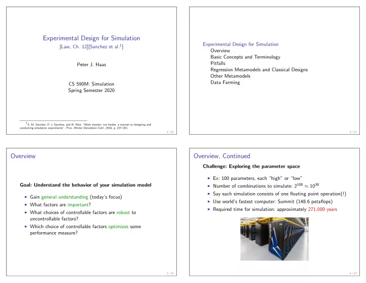
Experimental Design for Simulation Experimental Design for Simulation [Law, Ch. 12][Sanchez et al. 1 ] Overview Basic Concepts and Terminology Pitfalls Peter J. Haas Regression Metamodels and Classical Designs Other Metamodels Data Farming CS 590M: Simulation Spring Semester 2020 1S. M. Sanchez, P. J. Sanchez, and H. Wan. “Work smarter, not harder: a tutorial on designing and conducting simulation experiments”. Proc. Winter Simulation Conf. , 2018, p. 237–251. 1 / 23 2 / 23 Overview Overview, Continued Challenge: Exploring the parameter space ◮ Ex: 100 parameters, each “high” or “low” ◮ Number of combinations to simulate: 2 100 ≈ 10 30 Goal: Understand the behavior of your simulation model ◮ Say each simulation consists of one floating point operation(!) ◮ Gain general understanding (today’s focus) ◮ Use world’s fastest computer: Summit (148.6 petaflops) ◮ What factors are important? ◮ Required time for simulation: approximately 271,000 years ◮ What choices of controllable factors are robust to uncontrollable factors? ◮ Which choice of controllable factors optimizes some performance measure? 3 / 23 4 / 23

Basic Concepts: Factors Factors (simulation inputs) ◮ Have impact on responses (simulation outputs) Experimental Design for Simulation ◮ Levels: Values of a factor used in experiments Overview ◮ Factor taxonomy: Basic Concepts and Terminology ◮ Quantitative vs qualitative (can encode qualitative) Pitfalls ◮ Discrete vs continuous Regression Metamodels and Classical Designs ◮ Binary or not Other Metamodels ◮ Controllable vs uncontrollable Data Farming ◮ Factors must be carefully defined ◮ Ex: ( s , S )-inventory model ◮ Use ( s , S ) or ( s , S − s ) Factor type Example as the factors? quantitative (cont.) Poisson arrival rate quantitative (discr.) # of machines qualitative service policy (FIFO, LIFO, . . . ) binary (open,closed), (high,low),. . . controllable # of servers uncontrollable weather (sun, rain, fog) 5 / 23 6 / 23 Basic Concepts: Designs Design matrix ◮ One column per factor ◮ Each row is a design point Experimental Design for Simulation ◮ Contains a level for each factor Overview ◮ Level values determined by a domain expert ◮ Natural or coded design levels Basic Concepts and Terminology ◮ Can have multiple replications of the design Pitfalls Regression Metamodels and Classical Designs ◮ Especially in simulation! Other Metamodels Data Farming Design Factor settings point x 1 x 2 x 3 1 − 1 − 1 − 1 2 +1 − 1 − 1 3 − 1 +1 − 1 4 +1 +1 − 1 5 − 1 − 1 +1 6 +1 − 1 +1 7 − 1 +1 +1 8 +1 +1 +1 2 3 factorial design 7 / 23 8 / 23

Some Bad Designs: Capture the Flag Confounded effects ◮ Claim: Speed is the most important Experimental Design for Simulation ◮ Claim: Stealth is the most important Overview ◮ Claim: Both are equally important Basic Concepts and Terminology ◮ There is no way to determine who is right without more data Pitfalls ◮ Moral: haphazardly choosing design points can use up a lot of Regression Metamodels and Classical Designs time while not providing insight Other Metamodels Data Farming One-factor-at-a-time (OFAT) sampling ◮ Claim: Neither speed nor stealth is important ◮ Problem: an interaction between two factors is being missed 9 / 23 10 / 23 A Classical Design: 2 k Factorial Design Understanding Simulation Behavior: Metamodels Simulation metamodels approximate true response Basic setup: k factors with two levels each ( − 1 , +1 ) ◮ Simplified representation for greater insight ◮ Metamodel for k = 2: R ( x ) = β 1 x 1 + β 2 x 2 + β 12 x 1 x 2 + ǫ ◮ Allows ”simulation on demand” ◮ So r ( x ) = E [ R ( x )] = β 1 x 1 + β 2 x 2 + β 12 x 1 x 2 ◮ Allows factor screening and optimization Estimating “main effects” ◮ Avg. change in r when x 1 goes from − 1 to +1 ( x 2 fixed): Main-effects metamodel (quantitative factors) ( r 3 − r 1 )+( r 4 − r 2 ) = − r 1 − r 2 + r 3 + r 4 = r · x 1 = 2 β 1 R ( x ) = β 0 + β 1 x 1 + · · · + β k x k + ǫ ◮ 2 2 2 ◮ Similarly, r · x 2 2 = 2 β 2 Metamodel with second-order interaction effects ◮ Method-of-moments estimators: 2ˆ β 1 = R · x 1 and 2ˆ β 2 = R · x 2 2 2 R ( x ) = β 0 + β 1 x 1 + · · · + β k x k + � � j β ij x i x j + ǫ i Design Factor settings Observed Predicted point x 1 x 2 x 1 x 2 response ( R ) expected value ( r ) ◮ R = simulation model output (i.e., response) 1 − 1 − 1 +1 R 1 r 1 = − β 1 − β 2 + β 12 ◮ Factors x = ( x 1 , . . . , x k ) 2 − 1 +1 − 1 R 2 r 2 = − β 1 + β 2 − β 12 3 +1 − 1 − 1 R 3 r 3 = β 1 − β 2 − β 12 4 +1 +1 +1 R 4 r 4 = β 1 + β 2 + β 12 ◮ ǫ = mean-zero noise term, often assumed to be N (0 , σ 2 ) 11 / 23 12 / 23

2 k Factorial Design, Continued m k Designs Estimating “interaction effect” ◮ (Effect of ↑ x 1 with x 2 high minus effect with x 2 low) / 2 ( r 4 − r 2 ) − ( r 3 − r 1 ) = r · ( x 1 x 2 ) = 2 β 12 ◮ 2 2 ◮ Method of moments estimator: 2ˆ β 12 = R · ( x 1 x 2 ) 2 Observations: ◮ Can replicate design to get (Student-t) CI’s for coefficients ◮ Estimating effects ⇔ estimating regression coefficients ◮ Above analysis generalizes to more factors, e.g., Using more than two levels gives more detail ◮ E.g., capture the flag with 2 2 versus 11 2 designs R ( x ) = β 1 x 1 + β 2 x 2 + β 3 x 3 + β 12 x 1 x 2 + β 13 x 1 x 3 + β 23 x 2 x 3 + β 123 x 1 x 2 x 3 + ǫ ◮ After achieving a minimal level of stealth, speed is more important Design Factor settings Observed Predicted point response ( R ) expected value ( r ) x 1 x 2 x 1 x 2 ◮ Only possible for very small number of factors 1 − 1 − 1 +1 R 1 r 1 = − β 1 − β 2 + β 12 2 − 1 +1 − 1 R 2 r 2 = − β 1 + β 2 − β 12 3 +1 − 1 − 1 R 3 r 3 = β 1 − β 2 − β 12 4 +1 +1 +1 r 4 = β 1 + β 2 + β 12 R 4 13 / 23 14 / 23 2 k − p Fractional Factorial and Central Composite Designs Space-Filling Designs 2 k − p fractional factorial designs ◮ Fewer design points, carefully chosen (see Law, Table 12.17) ◮ E.g., 2 3 − 1 design with 4 design points Random Latin Hypercube design ◮ Left/right faces: 1 val. of x 2 at each level, 1 val. of x 3 at each level ◮ Based on random permutations of levels for each factor (can isolate x 1 effect) ◮ Similarly for other face pairs ◮ Good coverage of param. space w. relatively few design points ◮ The degree of confounding is specified by the resolution ◮ Carefully crafted LH designs are needed in practice ◮ No m -way and n -way effect are confounded if m + n < resolution ◮ So for Resolution V design, no main effect or 2-way interaction are confounded 15 / 23 16 / 23

Gaussian Metamodeling (Kriging) Ordinary kriging (deterministic simulations) ◮ Z ( x ) is a Gaussian process ◮ Models uncertainty due to interpolation extrinsic ◮ � � Z ( v 1 ) , Z ( v 2 ) , . . . , Z ( v n ) ∼ N ( 0 , R ( θ )) Experimental Design for Simulation uncertainty Overview ◮ r ( v i , v j ) = e − θ ( v i − v j ) 2 Basic Concepts and Terminology ˆ µ + r ⊤ ( x 0 ) R (ˆ θ ) − 1 ( Y − 1 ˆ Y ( x 0 ) = ˆ µ ) ◮ Pitfalls µ and ˆ ◮ ˆ θ are MLE estimates Regression Metamodels and Classical Designs ◮ Y = ( Y 1 , . . . , Y m ) and 1 = (1 , 1 , . . . , 1) Other Metamodels ◮ r = � r ( x 0 , x 1 ) , r ( x 0 , x 2 ) , . . . , r ( x 0 , x m ) Data Farming Stochastic kriging (stochastic simulations) ◮ ǫ is N (0 , σ 2 ) (“the nugget”) ◮ Captures simulation variability extrinsic + intrinsic ◮ Many other variants uncertainty ◮ Fitted derivatives ◮ Varying σ 2 ◮ Non-constant mean function 17 / 23 18 / 23 Kriging + Trees {speed:4, stealth:5, outcome:good} speed < 3 no Experimental Design for Simulation Overview stealth > 4 yes Basic Concepts and Terminology yes Pitfalls no stealth < 8 Regression Metamodels and Classical Designs no yes Other Metamodels Data Farming Kriging Model #1 Kriging Model #2 Kriging Model #3 Kriging Model #4 Idea: Build multiple models on subsets of homogeneous data ◮ Recursively split data to ◮ Maximize heterogeneity (e.g., Gini index) ◮ Maximize goodness of fit statistic (e.g., R 2 ) ◮ Build model on each subset 19 / 23 20 / 23

Data Farming Graphical Methods Modern “big data” approach Gaining insight through visualizations ◮ Unlike real-world experiments, easier to generate a lot of ◮ More sophisticated methods than simple regression simulation data ◮ Analyze flat areas (robustness) ◮ Most effort usually spent building model, so work it hard! ◮ Other characteristics of interest ◮ Use analytical, graphical, and data mining techniques on generated data 21 / 23 22 / 23 Data Mining and Visual Analytics Visual analytics ◮ Experiments are clustered based on system performance ◮ Parallel-coordinate plot relates performance to factor levels ◮ Ex: Manufacturing model with parameters P1, P2, P3, P4 N. Feldkamp, S. Bergmann, and S. Strassburger. Visual analytics of manufacturing simulation data. Proc. Winter Simulation Conference , 2015, pp. 779–790. 23 / 23