Experiment Latsis Symposium 2013, Zurich, 4th June 2013 - PowerPoint PPT Presentation
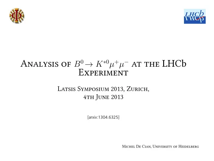
Michel De Cian, University of Heidelberg Experiment Latsis Symposium 2013, Zurich, 4th June 2013 [arxiv:1304.6325] Analysis of B 0 K 0 + at the LHCb . Particle . 2 . mass . 15 B 0 K 0 + decay topology K +
Michel De Cian, University of Heidelberg Experiment Latsis Symposium 2013, Zurich, 4th June 2013 [arxiv:1304.6325] Analysis of B 0 → K ∗ 0 µ + µ − at the LHCb
. Particle . 2 . mass . 15 B 0 → K ∗ 0 µ + µ − decay topology K + π − B 0 K ∗ 0 ds PV db µ + µ − lifetime ( cτ ) B 0 / c 2 5279 MeV 491 . 1 µ m K ∗ 0 / c 2 ≈ 3 · 10 − 12 µ m 892 MeV
. at the same level as SM physics. . 3 . distribution. . 15 B 0 → K ∗ 0 µ + µ − : Rare, but exciting d d d d ✁ ✁ W − B 0 K ∗ 0 u, ¯ c, ¯ t ¯ B 0 K ∗ 0 ¯ s b ¯ u, ¯ c, ¯ t ¯ ¯ s b ¯ Created by FeynDiag v0.1 Created by FeynDiag v0.1 W + W − ν µ γ, Z 0 µ − µ − µ + µ + • Rare decay with B = ( 1 . 05 +0 . 16 − 0 . 13 ) × 10 − 6 [PDG] • Decay only possible via penguin- or box diagrams, "new physics" can enter • Pseudoscalar → Vector-Vector decay: Plenty of observables in the angular
. Angular distribution (I) . 4 . form-factors. . 15 • Decay can be fully described by three angles ( θ ℓ , θ K , φ ) and the dimuon invariant mass (square) q 2 . 9 d 4 Γ 9 I ( s,c ) ∑ · f ( cos θ i , cos θ ℓ , φ ) . d cos θ ℓ d cos θ K d φ d q 2 = i 32 π i =1 • I i are function of Wilson-coefficients C ( ′ ) 7 , C ( ′ ) 9 , C ( ′ ) 10 and hadronic • In an ideal world, we would fit this expression to the collision data and extract all I i observables. • Can construct CP -symmetric and CP -antisymmetric observables: S i = I i + ¯ I i , A i = I i − ¯ I i ,
. Angular distribution (II) . 5 . 2011. . 15 This cancels four terms in the total angular distribution. enough for full angular fit. • In 2011, LHCb reconstructed ≈ 900 B 0 → K ∗ 0 µ + µ − events: Not • Apply "folding" technique: φ → φ + π for φ < 0 . • And leaves (neglecting lepton masses and S-wave contributions) d 4 (Γ + ¯ Γ) F L cos 2 θ K + 3 4 (1 − F L )(1 − cos 2 θ K ) + ∝ d cos θ ℓ d cos θ K d ϕ d q 2 F L cos 2 θ K (2 cos 2 θ ℓ ) + 1 4 (1 − F L )(1 − cos 2 θ K )(2 cos 2 θ ℓ − 1) + S 3 (1 − cos 2 θ K )(1 − cos 2 θ ℓ ) cos 2 ϕ + 4 3 A F B (1 − cos 2 θ K ) cos θ ℓ + A 9 (1 − cos 2 θ K )(1 − cos 2 θ ℓ ) sin 2 ϕ • This expression was fitted to the 1 fb − 1 of LHCb data at √ s = 7 TeV in
. Experimental aspects . 6 . simulation and collision data. correction, determined on simulation. . 15 LHCb ] 2 4 10 c ) [MeV/ 4000 3 10 3000 − µ + µ ( 10 2 m 2000 10 1000 0 1 5200 5400 5600 + π − µ µ − + 2 (K ) [MeV/ ] m c • Some experimental details: • Dominated by B 0 → J / ψ K ∗ 0 and B 0 → ψ (2 S ) K ∗ 0 in two regions: Cut out. • Peaking background due to misidentification of particles: Apply vetoes. • Select signal events with a BDT. • Acceptance of detector distorts angular distribution: Apply event-by-event • Correct for particle ID and efficiency (tracking, trigger, ...)-differences in • Perform a unbinned maximum-likelihood fit to the mass distribution and to ( θ ℓ , θ K , φ ) in 6 bins of q 2 .
. . . 7 . 15 Distribution of events in q 2 60 60 60 ) ) ) 2 2 2 c c c LHCb LHCb LHCb Candidates / ( 10 MeV/ Candidates / ( 10 MeV/ Candidates / ( 10 MeV/ 2 2 4 2 2 4 2 2 4 0.1 < q < 2 GeV / c 2 < q < 4.3 GeV / c 4.3 < q < 8.68 GeV / c 40 40 40 Signal Combinatorial bkg 20 Peaking bkg 20 20 0 0 0 5200 5400 5600 5200 5400 5600 5200 5400 5600 − − + π − µ µ − + π µ µ + π − µ µ − (K + ) [MeV/ 2 ] (K + ) [MeV/ 2 ] (K + ) [MeV/ 2 ] m c m c m c 60 60 60 ) ) ) 2 2 2 c c c LHCb LHCb LHCb Candidates / ( 10 MeV/ Candidates / ( 10 MeV/ Candidates / ( 10 MeV/ 2 2 4 2 2 4 2 2 4 10.09 < q < 12.86 GeV / c 14.18 < q < 16 GeV / c 16 < q < 19 GeV / c 40 40 40 20 20 20 0 0 0 5200 5400 5600 5200 5400 5600 5200 5400 5600 + π − µ µ − + π − µ µ − + π − µ µ − (K + ) [MeV/ 2 ] (K + ) [MeV/ 2 ] (K + ) [MeV/ 2 ] m c m c m c
. Results . 8 . Theory predictions from C. Bobeth et al.: [arXiv:1105.0376] . 15 Theory Binned Theory Binned LHCb LHCb 1 1 L FB F A LHCb LHCb 0.8 0.5 0.6 0 0.4 -0.5 0.2 0 -1 0 5 10 15 20 0 5 10 15 20 2 2 4 2 2 4 q [GeV / c ] q [GeV / c ] Theory Binned LHCb LHCb 3 9 A S 0.4 0.4 LHCb LHCb 0.2 0.2 0 0 -0.2 -0.2 -0.4 -0.4 0 5 10 15 20 0 5 10 15 20 2 2 2 4 2 4 q [GeV / c ] q [GeV / c ]
. Comparison with other experiments . 9 . BaBar: [PRD 86 (2012)] Belle: [PRL 103 (2009)] CDF: [PRL 108 (2012)] CMS: [CMS-BPH-11-009] ATLAS: [ATLAS-CONF-2013-038] Theory predictions from C. Bobeth et al.: [arXiv:1105.0376] . 15 Theory Binned Theory Binned LHCb CDF BaBar Belle ATLAS CMS LHCb CDF BaBar Belle ATLAS CMS 1 1 L FB F A 0.8 0.5 0.6 0 0.4 -0.5 0.2 0 -1 0 5 10 15 20 0 5 10 15 20 2 2 4 2 2 4 q [GeV / c ] q [GeV / c ] Theory Binned LHCb CDF LHCb CDF 1 1 T 9 2 A A 0.5 0.5 0 0 -0.5 -0.5 -1 -1 0 5 10 15 20 0 5 10 15 20 2 2 2 4 2 4 q [GeV / c ] q [GeV / c ]
. Measuring the zero-crossing point . 10 . factors cancel (to first order). [LHCb-CONF-2012-008] Backward Forward . 15 of A FB (I) ) ) 4 4 LHCb LHCb /c /c 2 15 2 15 Events / ( 0.2 GeV Preliminary Events / ( 0.2 GeV Preliminary 10 10 5 5 0 0 2 4 6 2 4 6 2 4 2 4 q 2 (GeV /c ) q 2 (GeV /c ) • Zero-crossing point of A F B is a very clean measurement, as the form • Zero-crossing point was extracted using "unbinned counting" technique: Make a 2D unbinned likelihood fit to ( q 2 , mass) for "forward" and "backward" events (with respect to cos θ ℓ ) . • Extract A F B = N F · P DF F ( q 2 ) − N B · P DF B ( q 2 ) N F · P DF F ( q 2 )+ N B · P DF B ( q 2 )
. Measuring the zero-crossing point values) [JHEP 1201 (2012) 107][Eur. Phys. J. C41 (2005), 173][Eur. Phys. J. C47 (2006) 625] . . 11 . 15 of A FB (II) • Standard Model theory predicts zero-crossing in 4.0 - 4.3 GeV 2 / c 4 (central • LHCb result: 4 . 9 ± 0 . 9 GeV 2 / c 4
. Clean observables . 12 . weighted average of the transverse observables. . . 15 are not affected by form-factor uncertainties. • Goal is to measure (more) observables which have a "clean" prediction, i.e. • Two examples: 2 (1 − F L ) A (2) • S 3 = 1 T 4 (1 − F L ) A ( Re ) • A F B = 3 T • Can re-express the angular distribution using these replacements and determine A (2) and A ( Re ) T T • Caveat: F L and A (2) T / A ( Re ) both vary with q 2 . Result presented is a T
. . . 13 . 15 A (2) T and A ( Re ) T Theory Binned Theory Binned LHCb LHCb 1 1 2 T Re A T A LHCb 0.5 0.5 0 0 -0.5 -0.5 LHCb -1 -1 0 5 10 15 20 0 5 10 15 20 2 2 4 2 2 4 q [GeV / c ] q [GeV / c ]
. More (clean) variables . 14 . . 15 measured 4 of them due to folding, measure the remaining ones as well. Descotes-Genon, et al. [JHEP05(2013)137] • Angular distribution has 8 independent observables in total. Have only • Instead of measuring the S i observables one can choose basis: { } d Γ dq 2 , F L , P 1 , ..., P 6 , with P 1 , ..., P 6 clean observables. • P 1 = A (2) T , P 2 = A ( Re ) T • Goal is to measure all observables of this basis. • From an experimental point it's advantageous to replace: P 4 , P 5 , P 6 with: P ′ 4 , P ′ 5 , P ′ 6
. Summary ). All agree with SM predictions. observables which are less affected by form-factor uncertainties. . . 15 . 15 • Performed an angular analysis of B 0 → K ∗ 0 µ + µ − and measured the observables F L , S 3 , A FB and A 9 (and A (2) and A ( Re ) T T • Measured the zero-crossing point of A FB . • The future is the determination of the "remaining" information, using
fin
. The LHCb detector . 17 . . 15 y Particle ID Tracking HCAL ECAL M5 M4 SPD/PS 5m M3 M2 Magnet RICH2 M1 T3 T2 T1 TT Vertex Locator p p 5m 10m 15m 20m z • b -quarks are produced in pairs, mostly in the forward- and backward region. • LHCb has excellent tracking capabilities ( ∆ p / p ≈ 0 . 4 − 0 . 6 %)... • ... and very good particle identification: K and π can be separated up to p ≈ 100 GeV / c . • Collected ≈ 1 fb − 1 in 2011 and ≈ 2.2 fb − 1 in 2012
. Differential branching fraction . 18 . . 15 Theory Binned LHCb 1.5 ] -2 GeV LHCb 4 c 1 × -7 [10 2 q 0.5 /d B d 0 0 5 10 15 20 2 2 4 q [GeV / c ]
. BDT input variables . . 19 . 15 • the B 0 pointing to the primary vertex, flight-distance and IP χ 2 with respect to the primary vertex, p T and vertex quality ( χ 2 ); • the K ∗ 0 and dimuon flight-distance and IP χ 2 with respect to the pri- mary vertex (associated to the B 0 ), p T and vertex quality ( χ 2 ); • the impact parameter χ 2 and the ∆ LL ( K − π ) and ∆ LL ( µ − π ) of the four final state particles.
Recommend
More recommend
Explore More Topics
Stay informed with curated content and fresh updates.
