Examples of Reinforcement Learning Robocup Soccer Teams Stone & - - PDF document

1

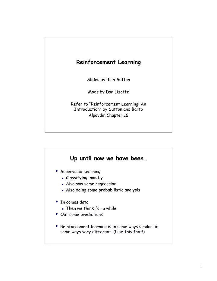
Reinforcement Learning

Slides by Rich Sutton Mods by Dan Lizotte Refer to “Reinforcement Learning: An Introduction” by Sutton and Barto Alpaydin Chapter 16

Up until now we have been…

• Supervised Learning

 Classifying, mostly  Also saw some regression  Also doing some probabilistic analysis

• In comes data

 Then we think for a while

• Out come predictions
• Reinforcement learning is in some ways similar, in

some ways very different. (Like this font!)

2

Complete Agent

• Temporally situated
• Continual learning and planning
• Objective is to affect the environment
• Environment is stochastic and uncertain

Environment action state reward Agent

What is Reinforcement Learning?

• An approach to Artificial Intelligence
• Learning from interaction
• Goal-oriented learning
• Learning about, from, and while interacting with an

external environment

• Learning what to do—how to map situations to

actions—so as to maximize a numerical reward signal

3

Chapter 1: Introduction

Psychology Artificial Intelligence Control Theory and Operations Research Artificial Neural Networks Reinforcement Learning (RL) Neuroscience

Key Features of RL

• Learner is not told which actions to take
• Trial-and-Error search
• Possibility of delayed reward

 Sacrifice short-term gains for greater long-

term gains

• The need to explore and exploit
• Considers the whole problem of a goal-directed

agent interacting with an uncertain environment

4

Examples of Reinforcement Learning

• Robocup Soccer Teams Stone & Veloso, Reidmiller et al.



World’s best player of simulated soccer, 1999; Runner-up 2000

• Inventory Management Van Roy, Bertsekas, Lee & Tsitsiklis



10-15% improvement over industry standard methods

• Dynamic Channel Assignment Singh & Bertsekas, Nie & Haykin



World's best assigner of radio channels to mobile telephone calls

• Elevator Control Crites & Barto



(Probably) world's best down-peak elevator controller

• Many Robots



navigation, bi-pedal walking, grasping, switching between skills...

• TD-Gammon and Jellyfish Tesauro, Dahl



World's best backgammon player

Supervised Learning

Supervised Learning System

Inputs Outputs Training Info = desired (target) outputs

Error = (target output – actual output)

5

Reinforcement Learning

RL System

Inputs Outputs (“actions”) Training Info = evaluations (“rewards” / “penalties”)

Objective: get as much reward as possible

Today

• Give an overview of the whole RL problem…

 Before we break it up into parts to study

individually

• Introduce the cast of characters

 Experience (reward)  Policies  Value functions  Models of the environment

• Tic-Tac-Toe example

6

Elements of RL

• Policy: what to do
• Reward: what is good
• Value: what is good because it predicts reward
• Model: what follows what

Policy Reward Value Model of environment

A Somewhat Less Misleading View…

external sensations

memory

state reward actions internal sensations RL agent

7

An Extended Example: Tic-Tac-Toe

X X X O O X X O X O X O X O X X O X O X O X O X O X O X

} x’s move

} x’s move } o’s move } x’s move

} o’s move ... ... ... ...

... ... ... ... ...

x x x x o x

• x
• x

x x x

• Assume an imperfect opponent:

—he/she sometimes makes mistakes

An RL Approach to Tic-Tac-Toe

• 1. Make a table with one entry per

state:

• 2. Now play lots of games.

To pick our moves, look ahead one step:

State V(s) – estimated probability of winning .5 ? .5 ? . . . . . . . . . . . . 1 win 0 loss . . . . . . 0 draw

x x x x

• x

x

• x

x x x

• current state

various possible next states

*

Just pick the next state with the highest estimated prob. of winning — the largest V(s); a greedy move. But 10% of the time pick a move at random; an exploratory move.

8

RL Learning Rule for Tic-Tac-Toe

“Exploratory” move

s – the state before our greedy move

• s – the state after our greedy move

We increment each V(s) toward V( s ) – a backup : V(s) V(s) + V( s ) V(s)

[ ]

a small positive fraction, e.g., = .1 the step - size parameter

• Our Move {

Opponent's Move { Our Move { Starting Position

• a

b c d e e' Opponent's Move {

• f
• g

Opponent's Move { Our Move {

• c

* * * g

How can we improve this T.T.T. player?

• Take advantage of symmetries

 representation/generalization  How might this backfire?

• Do we need “random” moves? Why?

 Do we need the full 10%?

• Can we learn from “random” moves?
• Can we learn offline?

 Pre-training from self play?  Using learned models of opponent?

• . . .

9

e.g. Generalization

Table Generalizing Function Approximator State V State V s s s . . . s

1 2 3 N

Train here

e.g. Generalization

Table Generalizing Function Approximator State V State V s s s . . . s

1 2 3 N

Train here

10

How is Tic-Tac-Toe Too Easy?

• Finite, small number of states
• One-step look-ahead is always possible
• State completely observable
• . . .

Chapter 2: Evaluative Feedback

• Evaluating actions vs. instructing by giving correct actions
• Pure evaluative feedback depends totally on the action taken.

Pure instructive feedback depends not at all on the action taken.

• Supervised learning is instructive; optimization is evaluative
• Associative vs. Nonassociative:

 Associative: inputs mapped to outputs;

– learn the best output for each input

 Nonassociative: “learn” (find) one best output

– ignoring inputs

• A simpler example: n-armed bandit (at least how we treat it) is:

 Nonassociative  Evaluative feedback

11

= Pause for Stats =

• Suppose X is a real-valued random variable
• Expectation (“Mean”)
• Normal Distribution

 Mean μ  Standard Deviation σ  Almost all values will be  -3σ < x < 3σ

E{X} = lim

n

x1 + x2 + x3 + ...+ xn n

The n-Armed Bandit Problem

• Choose repeatedly from one of n actions; each

choice is called a play

• After each play , you get a reward , where

at r

t

These are unknown action values ction values Distribution of depends only on

r

t

at

• Objective is to maximize the reward in the long

term, e.g., over 1000 plays To solve the n-armed bandit problem, you must explore xplore a variety of actions and exploit xploit the best of them

12

The Exploration/Exploitation Dilemma

• Suppose you form estimates
• The greedy action at t is at
• If you need to learn, you can’t exploit all the time;

if you need to do well, you can’t explore all the time

• You can never stop exploring; but you should always

reduce exploring. Maybe.

Qt(a) Q

*(a)

action value estimates action value estimates

at

* = argmax a Qt(a)

at = at

* exploitation

at at

* exploration

Action-Value Methods

• Methods that adapt action-value estimates and

nothing else, e.g.: suppose by the t-th play, action had been chosen times, producing rewards then

• ka

r

1, r 2, K, rka ,

“sample average”

lim

k a Qt(a) = Q *(a)

a

13

ε-Greedy Action Selection

• Greedy action selection:
• ε-Greedy:

at = at

* = arg max a Qt(a)

at

* with probability 1

random action with probability

{

at =

. . . the simplest way to balance exploration and exploitation

10-Armed Testbed

• n = 10 possible actions
• Each is chosen randomly from a normal

distribution with mean 0 and variance 1

• each is also normal, with mean Q*(at) and variance 1
• 1000 plays
• repeat the whole thing 2000 times and average the

results

• Use sample average to estimate Q

r

t

Q

*(a)

14

ε-Greedy Methods on the 10-Armed Testbed Softmax Action Selection

• Softmax action selection methods grade action
• probs. by estimated values.
• The most common softmax uses a Gibbs, or

Boltzmann, distribution:

• Actions with greater value are more likely to be

selected

Choose action a on play t with probability e

Qt (a)

eQt (b)

b=1 n

• ,

where is the

“computational temperature”

15

Softmax and ‘Temperature’

Choose action a on play t with probability e

Qt (a)

eQt (b)

b=1 n

• ,

where is the “computational temperature”

Q(a3) = -3.0 Q(a2) = 2.0 Q(a1) = 1.0 Probability ➘ 0.3234 0.3400 0.3366 τ = 100.0 0.2415 0.3982 0.3603 τ = 10.0 0.0049 0.7275 0.2676 τ = 1.0 < 0.0001 0.8808 0.1192 τ = 0.5 < 0.0001 0.9820 0.0180 τ = 0.25

Small τ is like ‘max.’ Big τ is like ‘uniform.’

Incremental Implementation

Qk = r

1 + r 2 +Lr k

k

Recall the sample average estimation method: Can we do this incrementally (without storing all the rewards)? We could keep a running sum and count, or, equivalently:

Qk+1 = Qk + 1 k +1 r

k+1 Qk

[ ]

The average of the first k rewards is (dropping the dependence on ):

This is a common form for update rules: NewEstimate = OldEstimate + StepSize[Target – OldEstimate]

a

16

Tracking a Nonstationary Problem

Choosing to be a sample average is appropriate in a stationary problem, i.e., when none of the change over time, But not in a nonstationary problem.

Qk

Q

*(a)

Better in the nonstationary case is:

Qk+1 = Qk + r

k+1 Qk

[ ]

for constant , 0 < 1 = (1 )

kQ0 +

(1

i =1 k

• )

k iri

exponential, recency-weighted average

Optimistic Initial Values

• All methods so far depend on , i.e., they are biased.
• Suppose instead we initialize the action values
• ptimistically,

Q0(a)

i.e., on the 10-armed testbed, use Q0(a) = 5 for all a

17

Conclusions

• These are all very simple methods

 but they are complicated enough—we will build on

them

 we should understand them completely

Conclusions

• These are all very simple methods

 but they are complicated enough—we will build on

them

 we should understand them completely

• Ideas for improvements:

 estimating uncertainties . . . interval estimation  new “action elimination” methods (see ICML’03)  approximating Bayes optimal solutions  Gittens indices

• The full RL problem offers some ideas for solution .

. .

 see work of Duff, e.g., at ICML’03, or Tao Wang

18

Chapter 3: The Reinforcement Learning Problem

• describe the RL problem we will be studying for the

remainder of the course

• present idealized form of the RL problem for which we

have precise theoretical results;

• introduce key components of the mathematics: value

functions and Bellman equations;

• describe trade-offs between applicability and

mathematical tractability.

Objectives of this chapter:

The Agent-Environment Interface

Agent and environment interact at discrete time steps : t = 0, 1, 2, K Agent observes state at step t: st S produces action at step t : at A(st ) gets resulting reward : r

t +1

and resulting next state : st +1

t

. . . st a rt +1 st +1 t +1 a rt +2 st +2

t +2

a rt +3 st +3 . . .

t +3

a

19

Policy at step t, t : a mapping from states to action probabilities t (s, a) = probability that at = a when st = s

The Agent Learns a Policy

• Reinforcement learning methods specify how the

agent changes its policy as a result of experience.

• Roughly, the agent’s goal is to get as much reward

as it can over the long run.

Getting the Degree of Abstraction Right

• Time steps need not refer to fixed intervals of real time.
• Actions can be low level (e.g., voltages to motors), or high

level (e.g., accept a job offer), “mental” (e.g., shift in focus

• f attention), etc.
• States can low-level “sensations”, or they can be abstract,

symbolic, based on memory, or subjective (e.g., the state of being “surprised” or “lost”).

• An RL agent is not like a whole animal or robot.
• Reward computation is in the agent’s environment because

the agent cannot change it arbitrarily.

• The environment is not necessarily unknown to the agent,
• nly incompletely controllable.

20

Goals and Rewards

• Is a scalar reward signal an adequate notion of a

goal?—maybe not, but it is surprisingly flexible.

• A goal should specify what we want to achieve, not

how we want to achieve it.

• A goal must be outside the agent’s direct

control—thus outside the agent.

• The agent must be able to measure success:

 explicitly;  frequently during its lifespan.

The reward hypothesis

• That all of what we mean by goals and purposes

can be well thought of as the maximization of the cumulative sum of a received scalar signal (reward)

• A sort of null hypothesis.

 Probably ultimately wrong, but so simple we

have to disprove it before considering anything more complicated

21

Returns

Suppose the sequence of rewards after step t is : r

t +1, rt+ 2, r t + 3, K

What do we want to maximize?

In general, we want to maximize the expected return, E Rt

{ }, for each step t.

Episodic tasks: interaction breaks naturally into episodes, e.g., plays of a game, trips through a maze.

R

t = rt +1 + rt +2 +L + r T ,

where T is a final time step at which a terminal state is reached, ending an episode.

Returns for Continuing Tasks

Continuing tasks: interaction does not have natural episodes. Discounted return:

R

t = r t +1 + rt+ 2 + 2r t +3 +L =

kr

t + k+1, k =0

• where , 0 1, is the discount rate

. shortsighted 0 1 farsighted

22

An Example

Avoid failure: the pole falling beyond a critical angle or the cart hitting end of track.

reward = +1 for each step before failure return = number of steps before failure

As an episodic task where episode ends upon failure: As a continuing task with discounted return:

reward = 1 upon failure; 0 otherwise return = k , for k steps before failure

In either case, return is maximized by avoiding failure for as long as possible.

Another Example

Get to the top of the hill as quickly as possible.

reward = 1 for each step where not at top of hill return = number of steps before reaching top of hill

Return is maximized by minimizing number of steps to reach the top of the hill.

23

A Unified Notation

• In episodic tasks, we number the time steps of

each episode starting from zero.

• We usually do not have to distinguish between

episodes, so we write instead of for the state at step t of episode j.

• Think of each episode as ending in an absorbing

state that always produces reward of zero:

• We can cover all cases by writing

st

st, j

Rt = kr

t +k+1, k= 0

• where can be 1 only if a zero reward absorbing state is always reached.

The Markov Property

• By “the state” at step t, the book means whatever

information is available to the agent at step t about its environment.

• The state can include immediate “sensations,” highly

processed sensations, and structures built up over time from sequences of sensations.

• Ideally, a state should summarize past sensations so as

to retain all “essential” information, i.e., it should have the Markov Property:

Pr st +1 = s , r

t +1 = r st ,at,r t, st 1,at 1,K,r 1,s0,a0

{ } =

Pr st +1 = s , r

t +1 = r st ,at

{ }

for all s , r, and histories st ,at,r

t, st 1,at 1,K,r 1, s0,a0.

24

Markov Decision Processes

• If a reinforcement learning task has the Markov Property, it is

basically a Markov Decision Process (MDP).

• If state and action sets are finite, it is a finite MDP.
• To define a finite MDP, you need to give:

 state and action sets  one-step “dynamics” defined by transition probabilities:  reward probabilities:

Ps

s a = Pr st +1 =

s st = s,at = a

{ } for all s,

s S, a A(s). Rs

s a = E r t +1 st = s,at = a,st +1 =

s

{ } for all s,

s S, a A(s).

Recycling Robot

An Example Finite MDP

• At each step, robot has to decide whether it should (1) actively

search for a can, (2) wait for someone to bring it a can, or (3) go to home base and recharge.

• Searching is better but runs down the battery; if runs out of

power while searching, has to be rescued (which is bad).

• Decisions made on basis of current energy level: high, low.
• Reward = number of cans collected

25

Recycling Robot MDP

S = high, low

{ }

A(high) = search, wait

{ }

A(low) = search, wait, recharge

{ }

Rsearch = expected no. of cans while searching Rwait = expected no. of cans while waiting Rsearch > Rwait

Value Functions

State - value function for policy : V

(s) = E R t

st = s

{ } = E

• kr

t +k +1 st = s k =0

• Action- value function for policy

: Q

(s, a) = E Rt st = s, at = a

{ } = E

• kr

t + k+1 st = s,at = a k= 0

• The value of a state is the expected return

starting from that state; depends on the agent’s policy:

• The value of taking an action in a state under

policy π is the expected return starting from that state, taking that action, and thereafter following π :

26

Bellman Equation for a Policy π

R

t = rt +1 + r t +2 + 2r t + 3 + 3r t + 4L

= rt +1 + rt +2 + r

t +3 + 2r t + 4L

( )

= rt +1 + Rt +1

The basic idea: So:

V

(s) = E R t st = s

{ }

= E rt +1 + V st +1

( ) st = s

{ }

Or, without the expectation operator: V (s) = (s,a) Ps

s a Rs s a + V (

s )

[ ]

• s
• a
• More on the Bellman Equation

V (s) = (s,a) Ps

s a Rs s a + V (

s )

[ ]

• s
• a
• This is a set of equations (in fact, linear), one for each state.

The value function for π is its unique solution. Backup diagrams:

for V

• for Q

27

Gridworld

• Actions: north, south, east, west; deterministic.
• If would take agent off the grid: no move but reward = –1
• Other actions produce reward = 0, except actions that move

agent out of special states A and B as shown. State-value function for equiprobable random policy; γ = 0.9

Golf

• State is ball location
• Reward of –1 for each stroke

until the ball is in the hole

• Value of a state?
• Actions:



putt (use putter)



driver (use driver)

• putt succeeds anywhere on

the green

28

• if and only if V

(s) V

• (s) for all s S

Optimal Value Functions

• For finite MDPs, policies can be partially ordered:
• There are always one or more policies that are better

than or equal to all the others. These are the optimal

• policies. We denote them all π *.
• Optimal policies share the same optimal state-value

function:

• Optimal policies also share the same optimal action-

value function: V

(s) = max

• V

(s) for all s S

Q

(s, a) = max

• Q

(s, a) for all s S and a A(s)

This is the expected return for taking action a in state s and thereafter following an optimal policy.

Optimal Value Function for Golf

• We can hit the ball farther with driver than with

putter, but with less accuracy

• Q*(s,driver) gives the value or using driver first,

then using whichever actions are best

29

Bellman Optimality Equation for V*

V (s) = max

aA(s)Q (s,a)

= max

aA(s)E r t +1 + V (st +1) st = s,at = a

{ }

= max

aA(s)

Ps

s a

• s
• Rs

s a + V (

s )

[ ]

The value of a state under an optimal policy must equal the expected return for the best action from that state: The relevant backup diagram: is the unique solution of this system of nonlinear equations.

V

• Bellman Optimality Equation for Q*

Q(s,a) = E r

t +1 + max

• a Q(st +1,

a ) st = s,at = a

{ }

= Ps

s a Rs s a + max

• a Q(

s , a )

[ ]

• s
• The relevant backup diagram:

is the unique solution of this system of nonlinear equations.

Q

*

30

Why Optimal State-Value Functions are Useful

V

• V
• Any policy that is greedy with respect to is an optimal policy.

Therefore, given , one-step-ahead search produces the long-term optimal actions. E.g., back to the gridworld:

π*

What About Optimal Action-Value Functions?

Given , the agent does not even have to do a one-step-ahead search:

Q

*

• (s) = arg max

aA(s) Q (s, a)

31

Solving the Bellman Optimality Equation

• Finding an optimal policy by solving the Bellman Optimality

Equation requires the following:

 accurate knowledge of environment dynamics;  we have enough space and time to do the computation;  the Markov Property.

• How much space and time do we need?

 polynomial in number of states (via dynamic programming

methods; Chapter 4),

 BUT, number of states is often huge (e.g., backgammon

has about 1020 states).

• We usually have to settle for approximations.
• Many RL methods can be understood as approximately

solving the Bellman Optimality Equation.

Summary

• Agent-environment interaction



States



Actions



Rewards

• Policy: stochastic rule for

selecting actions

• Return: the function of future

rewards agent tries to maximize

• Episodic and continuing tasks
• Markov Property
• Markov Decision Process



Transition probabilities



Expected rewards

• Value functions

 State-value function for a

policy

 Action-value function for a

policy

 Optimal state-value function  Optimal action-value function

• Optimal value functions
• Optimal policies
• Bellman Equations
• The need for approximation