Example: the binary tree of Example 2.1.2: The outcomes are the 8 - PowerPoint PPT Presentation
Martingales Mathematical background of random variables and stochastic processes: A sample space with outcomes ; A collection of subsets F ; F is a -field; F , and F is closed under complementation and
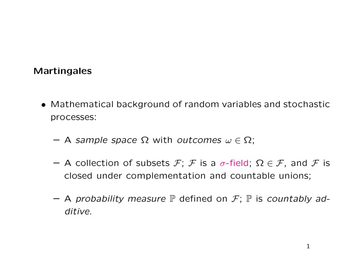
Martingales • Mathematical background of random variables and stochastic processes: – A sample space Ω with outcomes ω ∈ Ω; – A collection of subsets F ; F is a σ -field; Ω ∈ F , and F is closed under complementation and countable unions; – A probability measure P defined on F ; P is countably ad- ditive . 1
• Axioms of probability: – 0 ≤ P [ A ] ≤ 1 for all A ∈ F ; – P [Ω] = 1; – P [ A ∪ B ] = P [ A ] + P [ B ] for any disjoint A, B ∈ F ; – If A n ∈ F for all n ∈ N and A 1 ⊆ A 2 ⊆ . . . , then P [ A n ] ↑ P [ n A n ] as n ↑ ∞ . � • These imply countable additivity: if B n ∈ F for all n ∈ N and { B n } are disjoint , then P [ n B n ] = � n P [ B n ]. � 2
• Example: the binary tree of Example 2.1.2: • The outcomes are the 8 possible paths from t = 0 to t = T . • That is, Ω = { uuu, uud, udu, udd, duu, dud, ddu, ddd } , (or equiv- alently { 000 , 001 , 010 , 011 , 100 , 101 , 110 , 111 } ). • F is the power set 2 Ω : the collection of all subsets of Ω. 3
• Random variable: a real-valued function X on Ω that is F - measurable : { ω ∈ Ω : X ( ω ) ≤ x } ∈ F for all x ∈ R ; – that is, the probability P [ X ≤ x ] = P [ { ω ∈ Ω : X ( ω ) ≤ x } ] is defined. • The cumulative distribution function of X is F ( x ) = P [ X ≤ x ] . 4
• Example: the binary tree. • Because Ω is discrete and F = 2 Ω , every real-valued function on Ω is measurable. • Define X 1 and X 2 on Ω by X 1 ( uuu ) = X 1 ( uud ) = X 1 ( udu ) = X 1 ( udd ) = 120 , X 1 ( duu ) = X 1 ( dud ) = X 1 ( ddu ) = X 1 ( ddd ) = 80 , X 2 ( uuu ) = X 2 ( uud ) = 140 , X 2 ( udu ) = X 2 ( udd ) = 100 , X 2 ( duu ) = X 2 ( dud ) = 100 , X 2 ( ddu ) = X 2 ( ddd ) = 60 . and similarly X 3 . 5
• Note that X 1 is also measurable with respect to F 1 = { Ω , ∅ , { uuu, uud, udu, udd } , { duu, dud, ddu, ddd }} = { Ω , ∅ , { X 1 = 120 } , { X 1 = 80 }} ⊂ F . • We can similarly construct F 2 , with F 1 ⊂ F 2 ⊂ F , such that X 2 is F 2 -measurable, as well as F -measurable. 6
• A filtration is a σ -field F and a sequence of sub-fields {F n } with F n ⊆ F n +1 ⊆ · · · ⊆ F . • A stochastic process is a sequence of random variables { X n } n ≥ 0 on Ω. • The stochastic process { X n } n ≥ 0 is adapted to the filtration {F n } if X n is F n -measurable for each n ≥ 0. • Note that the definition of a stochastic process and its adap- tation do not depend on the existence of any probability measure P . 7
• Conditional expectation: – After one step in the tree, the remaining possible paths form a subtree. – We can define risk-neutral probabilities on the subtree, and hence the conditional expectation of the claim X 3 : E [ X 3 | X 1 = 120] and E [ X 3 | X 1 = 80]. • The conditional expectation is a function of X 1 , and therefore a random variable, measurable with respect to F 1 . 8
• The formal definition is less obvious: – Suppose that X is F -measurable with E [ | X | ] < ∞ and G ⊆ F is a sub- σ -field. – The conditional expectation of X given G is a G -measurable random variable E [ X |G ] such that, for any A ∈ G , � � A E [ X |G ] d P = A Xd P . • The conditional expectation always exists and is essentially unique. 9
• The “tower property:” if F i ⊆ F j , then E [ E [ X |F j ] |F i ] = E [ X |F i ] . • That is, we can calculate conditional expectation in steps: – First condition on detailed information ( F j ); – Then take the expected value conditional on less informa- tion ( F i ). • “Taking out what is known:” if E [ | X | ] < ∞ and E [ | XY | ] < ∞ , and Y is F n -measurable, then E [ XY |F n ] = Y E [ X |F n ] . 10
� � • Martingale: Suppose that Ω , {F n } n ≥ 0 , F , P is a filtered prob- ability space. The stochastic process { X n } n ≥ 0 adapted to {F n } is a martingale with respect to this space if, for any n ≥ 0, E [ | X n | ] < ∞ and E [ X n +1 |F n ] = X n . • On the binomial tree with zero interest rate, both S n and the price of the option are martingales. • With positive interest, the martingales are the discounted S n = e − rnδt S n and the discounted option price. stock price ˜ 11
� � • Conditional expectation of a claim: as before, Ω , {F n } n ≥ 0 , F , P is a filtered probability space (not necessarily a binary tree). If C N is F N -measurable with E [ | C N | ] < ∞ , and X n = E [ C N |F n ] , � � then { X n } 0 ≤ n ≤ N is a P , {F n } 0 ≤ n ≤ N -martingale. • More generally, if V n = e − r ( N − n ) δt E [ C N |F n ] is the expected value of the claim, discounted from t = N to t = n , and V n = e − rnδt V n ˜ is V n discounted from t = n to t = 0, then { ˜ V n } 0 ≤ n ≤ N is a � � P , {F n } 0 ≤ n ≤ N -martingale. 12
• New martingales from old. In the binary tree model for pric- ing a European option, we write ( φ n , ψ n ) for the amounts of stock and cash held for the time step [( n − 1) δt, nδt ). • If V n is the value of the portfolio at t = nδt , then V n = φ n +1 S n + ψ n +1 B n and because the strategy is self-financing, φ n +1 S n + ψ n +1 B n = φ n S n + ψ n B n or φ n +1 ˜ S n + ψ n +1 = φ n ˜ S n + ψ n . 13
• So � � V n +1 − ˜ ˜ S n +1 − ˜ ˜ V n = φ n +1 S n and, summing, n − 1 � � V n − ˜ ˜ S j +1 − ˜ ˜ � V 0 = φ j +1 S j . j =0 • We can verify directly that { ˜ V n } is a martingale, using the fact that φ n is known at time ( n − 1) δt ( φ n is F n − 1 -measurable). Such a process { φ n } n ≥ 1 is called {F n } n ≥ 0 -predictable or {F n } n ≥ 0 - previsible. 14
• In general, if { X n } n ≥ 0 is a ( P , {F n } n ≥ 0 )-martingale and { φ n } n ≥ 1 is {F n } n ≥ 0 -previsible, then n − 1 � � � Z n = Z 0 + X j +1 − X j φ j +1 , j =0 where Z 0 is a constant, is also a ( P , {F n } n ≥ 0 )-martingale. • We can view this sum as a discrete stochastic integral . 15
• Key theorem: Consider a more general multi-period market model with several assets. • No arbitrage: in this market model, there is no arbitrage if and only if there is a measure Q such that the discounted stock price vector is a Q -martingale. • In that case, the market price at t = 0 of an attainable claim C N at t = Nδt is unique and is given by E Q [ ψ 0 C N ] where 1 ψ ( i ) ψ 0 = � N is the discount factor over N periods. 0 • Q is the equivalent martingale measure . 16
Recommend
More recommend
Explore More Topics
Stay informed with curated content and fresh updates.


